mileages.txt.In this case you can store your data into the variable myData as follows.
| myData = read.csv('mileages.txt') |
It is a common task in statistics to compare two means or two proportions. In this lesson you will learn how to compare two means using confidence intervals and hypothesis tests. We assume throughout this lesson that we are sampling from a normal population.
Let's start with an example.
Is there a difference in body temperature between men and women? If so, what is the difference?
For a more precise formulation of this question, denote the mean body temperature of men by \(\mu_M\) and the mean body temperature of women by \(\mu_W.\) We are then interested in testing \[\begin{align*}& H_0: \quad \mu_W=\mu_M \quad \mbox{ versus }\\ & H_A: \quad \mu_W\neq\mu_M,\end{align*}\] and in finding confidence intervals for the difference \(\mu_W-\mu_M.\)
The hypothesis test formulated above could also be written as follows: \[\begin{align*}& H_0: \quad \mu_W-\mu_M=0\\ & H_A: \quad \mu_W-\mu_M \neq 0.\end{align*}\] Writing the test in this form motivates the appropriate test statistic. In the one sample t-test the hypothesis test was of the following form: \[\begin{align*}& H_0: \quad \mbox{parameter}=\mbox{hypothesized value} \\ & H_A: \quad \mbox{parameter}\neq\mbox{hypothesized value}.\end{align*}\] The type of test we want to do is of the same form! The only difference is that the parameter is \(\mu_W-\mu_M\) and the hypothesized value is 0.
The test statistic for the one-sample t-test is of the form \[ T=\frac{\mbox{estimate}-\mbox{hypothesized value}}{\mbox{SE(estimate)}}, \] where SE(estimate) denotes the standard error of the estimate.
A natural choice for a point-estimate of \(\mu_W-\mu_M\) is \(\bar{x}_W-\bar{x}_M,\) where \(\bar{x}_W\) and \(\bar{x}_M\) denote the sample means of women and men. Therefore, we guess that the appropriate test statistic is given by \[ T=\frac{\bar{x}_W-\bar{x}_M}{SE(\bar{x}_W-\bar{x}_M)}. \] We need to find \(SE(\bar{x}_W-\bar{x}_M)\). If the samples are independent, then \[\begin{align*} Var(\bar{x}_W-\bar{x}_M) & = Var(\bar{x}_W)+Var(\bar{x}_M)\\ & = \frac{\sigma_W^2}{n_W}+\frac{\sigma_M^2}{n_M},\end{align*}\] where \(\sigma_W^2\) and \(\sigma_M^2\) denote the variances of body temperatures in the population of women, and the population of men, and \(n_W\) and \(n_M\) denote the respective sample sizes.
The standard deviation of the estimate \(\bar{x}_W-\bar{x}_M\) is the square root of the variance, that is, \[ SD(\bar{x}_W-\bar{x}_M) = \sqrt{\frac{\sigma_W^2}{n_W}+\frac{\sigma_M^2}{n_M}}.\] The standard error of the estimate \(\bar{x}_W-\bar{x}_M\) is the estimated standard deviation of the estimate, which is \[ SE(\bar{x}_W-\bar{x}_M) = \sqrt{\frac{s_W^2}{n_W}+\frac{s_M^2}{n_M}},\] where \(s_W\) and \(s_M\) denote the sample standard deviations for women and men.
Unfortunately, the statistic \[ T=\frac{\bar{x}_W-\bar{x}_M}{\sqrt{\frac{s_W^2}{n_W}+\frac{s_M^2}{n_M}}} \] is not t-distributed. It turns out however, that the distribution of \(T\) is approximately t-distributed with \[ df = \frac{\left(\frac{s_W^2}{n_W}+\frac{s_M^2}{n_M}\right)^2}{ \frac{(s_W^2/n_W)^2}{n_W-1}+\frac{(s_M^2/n_M)^2}{n_M-1}} \] degrees of freedom. This equation is known as the Welch-Satterthwaite equation and the test using this test statistic \(T\) is called Welch's t-test.
Suppose that the variances for body temperatures for men and women are the same, that is, \(\sigma^2_W=\sigma^2_M.\) Denote the common variance by \(\sigma^2 .\) In this case , \[ \begin{align*} SD(\bar{x}_W-\bar{x}_M) & = \sqrt{\frac{\sigma^2}{n_W}+\frac{\sigma^2}{n_M}}\\ & = \sigma \sqrt{\frac{1}{n_W}+\frac{1}{n_M}}. \end{align*}\] Since both, \(s_W^2\) and \(s_M^2\), are estimates of \(\sigma^2\), we can combine \(s_W^2\) and \(s_M^2\) to form an estimate of \(\sigma^2 .\) How should we do that?
If the sample sizes are the same, then it would be reasonable to average the two estimates. If the sample sizes are not the same, then one expects the estimate based on the larger sample size to be closer to the true variance. It turns out that the best thing to do is to form a weighted average, which is weighted by the degrees of freedom of each estimate. In particular, the variance \(\sigma^2\) is estimated by the pooled variance \[\begin{align*} s_p^2 & = \left(\frac{n_W-1}{(n_W-1)+(n_M-1)}\right)s^2_W+\left(\frac{n_M-1}{(n_W-1)+(n_M-1)}\right)s^2_M\\ & = \frac{(n_W-1)s^2_W+(n_M-1)s^2_M}{n_W+n_M-2}.\end{align*}\] In this case, where \(\sigma^2_W=\sigma^2_M ,\) the test statistic \[ T=\frac{\bar{x}_W-\bar{x}_M}{s_p \sqrt{\frac{1}{n_W}+\frac{1}{n_M}}} \] is t-distributed with \(df = n_W+n_M-2\) degrees of freedom.
Recall that the two-sided confidence interval for a single mean has the following form: \[\mbox{estimate} \pm \mbox{critical value}\times \mbox{standard error}\]
The estimate for \(\mu_W-\mu_M\) is \(\bar{x}_W-\bar{x}_M \) and the standard error of this estimate is: \[ SE(\bar{x}_W-\bar{x}_M )=\left\{ \begin{array}{ll} s_p \sqrt{\frac{1}{n_W}+\frac{1}{n_M}} & \mbox{if } \sigma^2_W=\sigma^2_M \\ \sqrt{\frac{s_W^2}{n_W}+\frac{s_M^2}{n_M}} & \mbox{if } \sigma^2_W\neq\sigma^2_M \end{array} \right. \] A two-sided confidence interval is then given by \[\bar{x}_W-\bar{x}_M \pm t^{\star} SE(\bar{x}_W-\bar{x}_M )\] where the critical value \(t^{\star}\) depends on the confidence level \(C\) and the degrees of freedom \(df, \) which is either given by \(n_W+n_M-2\) when the variances are equal or by the Welch-Satterthwaite equation when the variances are not equal.
Suppose you formed pairs, each consisting of one woman and one man, where the two subjects are alike in all aspects that appear to be important with regard to body temperature - with the exception of gender. Suppose you measured the body temperature of each person and recorded the difference in temperature between the woman and man in each pair.
In this case we can apply the one-sample t-tools to the sample of differences, provided that the differences are normally distributed or that the sample sizes are sufficiently large.
Note that the expected value or mean of the differences in this case is \(\mu_W-\mu_M.\)
Is it better to compare the body temperatures of women and men by forming pairs or by taking independent random samples?
It all depends. If body temperature doesn't depend much on variables other than gender, then independent random samples should be taken because we loose degrees of freedom by forming pairs. On the other hand, if, for example, weight matters, then forming pairs of equal weight reduces the variation in temperature that is due to the weight, and typically this reduction in variance more than compensates for the loss of degrees of freedom.
Welch’s t-test is a robust alternative to the standard t-test that does not assume equal variances. However, it still relies on the assumption of normality. When the normality assumption is violated or when outliers are present, the Wilcoxon rank-sum test (also known as the Mann–Whitney U test) provides a nonparametric alternative. If the group distributions have similar shapes, this test can be interpreted as a test of medians. Otherwise, it serves as a test for stochastic dominance — that is, whether one distribution tends to produce larger values than the other. The permutation test offers another option and remains valid even when no specific distributional assumptions can be made.
I recommend that you use the R function t.test() to perform hypothesis tests and calculate confidence intervals. Here is an example.
Suppose that you have two cars and you want to know if there is a difference in the mileage you get between the two cars. Suppose that both cars hold 10 Gallons of gas and that the miles driven on a full tank are normally distributed for each car.
Let's say for car 1 you record 212, 228, 224, 232, and 250 miles and for car 2 you record 227, 268, 259, 236, and 262 miles.
Let's store the miles of car 1 in the variable car1
and store the miles of car 2 in the variable car2.
| car1 = c(212, 228, 224, 232, 250) |
| car2 = c(227, 268, 259, 236, 262) |
We can then perform the test \[H_0: \mu_1 = \mu_2 \quad \mbox{ versus }\quad H_A: \mu_1 \neq \mu_2\] and calculate a 95% confidence interval of \(\mu_1 - \mu_2\) with a single line of code.
| t.test(car1, car2) |
You can change the confidence level and the alternative hypothesis by setting the appropriate options in t.test(); type ?t.test into the R-console to find out about all available options. The results are based on Welch's t-test by default. With the option var.equal=T,
the results are obtained using the pooled variance.
For example, a 90% upper-bound confidence interval of \(\mu_1-\mu_2\) and the p-value for the test \[H_0: \mu_1 \geq \mu_2 \quad \mbox{ versus }\quad H_A: \mu_1 \lt \mu_2\] can be found with the following code.
| t.test(car1, car2, conf.level=0.9, alternative='less') |
Suppose you obtained the miles by having two drivers drive the cars the same route at the same time. In that case it would be best to do a paired t-test. Since
| car1-car2 |
produces the differences in the miles, you can perform a paired t-test with
| t.test(car1-car2) |
Alternatively, you can use the option paired=T
in the function t.test().
| t.test(car1, car2, paired=T) |
Typically, the data are collected in a spreadsheet. Suppose the data resides in the comma separated text file mileages.txt.In this case you can store your data into the variable myData as follows.
|
|
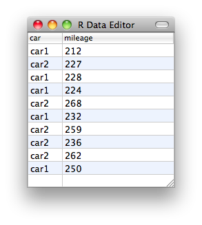
Just for demonstration purposes, we create the data frame myData as follows:
| myData <- data.frame( car = factor(rep(c("car1", "car2"), each = 5)), mileage = c(car1, car2) ) |
The following code calculates confidence intervals and performs hypothesis tests.
| t.test(mileage~car, data=myData) |
Note that the format mileage~car
is the same one that you used in simple linear regression. The variable mileage
is thought of as the response variable to the explanatory variable car.
The Wilcoxon rank-sum test can be performed as follows:
| wilcox.test(car1, car2, conf.level=0.9, alternative='less', conf.int = TRUE) |
Here is the code for the permutation test:
| library(coin) |
| oneway_test(mileage ~ car, data = myData, alternative='less', distribution = approximate(nresample = 10000)) |
This permutation test can be extended to calculate confidence intervals, but it’s not built into the basic implementation of the test in many R functions.
Download the file data.csv (comma separated text file) and read the data into R using the function read.csv(). Your data set consists of 100 measurements of body temperatures from women and men. Use the function t.test() to answer the following questions. Do not assume that the variances are equal.
Denote the mean body temperature of females and males by \(\mu_F\) and \(\mu_M\) respectively.
(b) Are the body temperatures for men and women significantly different?