A probability density function must be nonnegative and the area under the graph of \(y=f(x)\) has to be 1. | 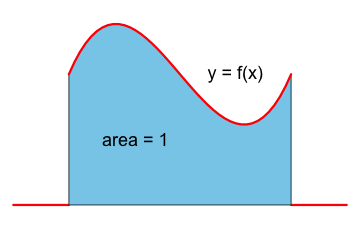 |
The probability of the event \(X\in A\) is given by the area under the graph of \(y=f(x)\) over the set \(A.\) |  |
In this lesson you will learn about continuous random variables, the Law of Large Numbers, and some general rules for finding the expected value and variance of linear combinations of random variables.
Consider the random experiment of growing a certain kind of tomatoes. Suppose you are particularly interested in the weight of a single tomato. Denote by \(W\) the random variable that assigns to each outcome of the sample space, a single tomato, its weight. Then the random variable \(W\) can assume all values in some interval of the real numbers. In this case the random variable \(W\) is called a continuous random variable.
What is the sample space \(S\), the set of all possible outcomes in our tomato experiment? This is hard to say, especially if you want to be precise. Luckily, we don't have to specify the sample space if we use random variables. All we need to know are the distributions of the random variables.
Let \(X\) be a continuous random variable. In this case \(X\) is specified by a probability density function \(f(x).\)
A probability density function must be nonnegative and the area under the graph of \(y=f(x)\) has to be 1. | |
The probability of the event \(X\in A\) is given by the area under the graph of \(y=f(x)\) over the set \(A.\) | |
If the set \(A\) is a very narrow interval then the probability that \(X\) will fall into the interval \(A\) is very small, since the area under the density function is small. In particular, when \(A\) contains just a single point then the probability will be 0, that is, \(P(X=x) = 0\) for all values of \(x.\)
In practice, we describe complex real world situations with random variables of specified distributions. This description typically involves simplification and approximation. We may decide, for example, that the weight of the tomato is normally distributed. This would be an approximation because every normal distribution can have negative values while the weight of a tomato is always positive.
The precise definition of the expected value of a continuous random variable requires some knowledge of calculus and will not be given here. The expected value of a random variable \(X,\) discrete or continuous, is denoted by \(E(X),\) \(\mu_X, \) or just \(\mu. \)
| The mean \(\mu\) of a continuous random variable \(X\) can be visualized as the location where the area under the probability density function, if it were made from some solid material, would balance. | 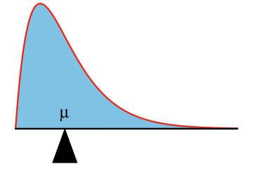
|
The variance of a continuous random variable is the expected value of the squared deviation of the random variable from its mean.
The variance of a random variable \(X\) is denoted by \(Var(X),\) \(\sigma^2_X,\) or just \(\sigma^2.\) It is defined by \[Var(X) = E\left[\left(X-\mu_X\right)^2\right].\] The standard deviation of a random variable \(X\) is denoted by \(\sigma_X\) or just \(\sigma.\) It is the square root of the variance of the random variable \(X.\)
Regardless of whether \(X\) is discrete or continuous, if \(X\) is interpreted as the amount won
in a game, then the value \(E(X)\) can be interpreted as the average amount won
in a single game when playing the game a very large number of times. This interpretation is a consequence of the Law of Large Numbers.
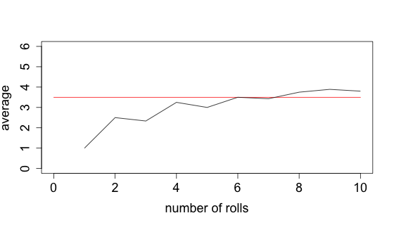
The Law of Large Numbers is a theorem which roughly speaking says that if you perform the same random experiment a large number of times, then the average of the results obtained should be close to the mean of the random variable describing the outcome of the experiment. Furthermore, the average will tend to get closer to the mean as more random experiments are performed.
As an illustration of the Law of Large Numbers, we can simulate the roll of a single die many times and plot the average score obtained in the first \(k\) rolls versus \(k.\) Click on the image below to change the number of rolls.
Suppose that after rolling the die 100 times your average score is 4. One might think that in order to get back to the mean, which is 3.5, it has to be more likely to roll the numbers 1, 2, or 3 than the numbers 4, 5, and 6. This is known as the gambler's fallacay or in lay terms as the law of averages.
This mistaken belief is also the reason why it is sometimes said that a person is now due
for success.
Here is the true reason why in the long run the average will be close to the expected value of 3.5. Even if after 100 rolls the average is 4, the average of these 100 rolls together with say 10,000 rolls that are close to 3.5, is also close to 3.5. \[\frac{100\cdot 4 + 10,000\cdot 3.5}{10,100}\approx 3.505\] And even if after 10,000 rolls the average were still 4, then the average of these 10,000 rolls together with another 10 billion rolls close to 3.5, would again be close to 3.5. \[\frac{10,000\cdot 4 + 10,000,000,000\cdot 3.5}{10,000,010,000}\approx 3.5000005\]
The Law of Large Numbers can also be used to justify the relative frequency interpretation of probability since the probability of an event described by a random variable \(X\) can always be written as the expected value of some random variable \(Y\).
In the following, \(X\) and \(Y\) denote random variables, and \(a\) and \(b\) denote some numbers. Here are some rules about expected values and variances that you need to know.
For our purposes it suffices to say that two random variables are independent if some information about one of them will not give any information about the other.
Denote by \(L\) the linear transformation \(L(x)=a +bx.\) The rule \(E[a + bX]=a + bE[X]\) can then be written as \(E[L(X)]=L(E[X]).\) In words, the expected value of a linear transformation is the linear transformation of the expected value.
Suppose that the random variable \(X\) is the body temperature measured in Fahrenheit of a randomly selected person from some population, and the linear transformation describes the change from Fahrenheit to Celsius. In this context this rule says that the mean of the measurement in Celsius is the same as the mean of the measurement in Fahrenheit converted to Celsius.
Suppose a random experiment consists of randomly selecting a person from a population and measuring \(X\), the low-density lipoprotein (LDL or bad
cholesterol) and \(Y\), the high-density lipoprotein (HDL or good
cholesterol). The rule \(E[X+Y]=E[X]+E[Y]\) then says that the mean of the sum of HDL and LDL is the same as the sum of the mean of HDL and the mean of LDL. If \(X\) and \(Y\) denote the winnings in two consecutive games, then \(E[X+Y]\) is the expected winning by playing both games, which is equal to the expected winning \(E[X]\) of the first game and the expected winning \(E[Y]\) of the second game. This rule can be extended to more than two random variables. The expected value of a sum of random variables is the sum of the expected values of the random variables.
Recall the definition of the variance: \(Var(X) = E[(X-\mu_X)^2]\). Let \(Y=a+bX.\) Then \[\begin{align} Var(a+bX) = Var(Y) & = E[(Y-\mu_Y)^2] \\ & = E[((a+bX)-(a+b\mu_X))^2]\\ & = E[(bX-b\mu_X)^2] \\ & = E[b^2(X-\mu_X)^2]\\ & = b^2 E[(X-\mu_X)^2]\\ & = b^2 Var(X)\end{align} \]
The rule that for independent random variables \(X\) and \(Y,\) \(Var(X+Y)=Var(X)+Var(Y),\) is not intuitive. This rule can also be generalized to more than two random variables. The variance of a sum of random variables is the sum of the variances of the random variables, provided that the variables are independent.
Suppose \(X\) and \(Y\) are random variables such that \(E[X]=2\) and \(E[Y]=3.\) Find \(E[2-X]\) and \(E[3X-2Y].\)
\[ \begin{align} E[2-X] & = E[2+ (-1)X] \\ & = 2 + (-1) E[X]\quad (\mbox{using }E[a + bX]=a + bE[X]) \\ & = 2 + (-1)2 = 0\end{align}\]
\[ \begin{align} E[3X-2Y] & = E[3X+(-2)Y] \\ & = E[3X]+E[(-2)Y] \quad (\mbox{using }E[X+Y]=E[X]+E[Y]) \\ & = 3E[X] + (-2)E[Y]\quad (\mbox{using }E[a + bX]=a + bE[X]) \\ & = 3\cdot 2 + (-2)\cdot 3 = 0\end{align}\]
Suppose \(X\) and \(Y\) are independent random variables such that \(Var(X)=1\) and \(Var(Y)=4.\) Find \(Var(X-Y)\) and \(Var(3X-2Y).\)
\[ \begin{align} Var(X-Y) & = Var(X +(-1)Y) \\ & = Var(X)+ Var((-1)Y) \quad (\mbox{using }Var(X+Y)=Var(X)+Var(Y)) \\ & = Var(X)+ (-1)^2Var(Y) \quad (\mbox{using }Var(a+bX)=b^2Var(X)) \\ & = Var(X) + Var(Y) = 1+4 = 5\end{align}\]
\[ \begin{align} Var(3X-2Y) & = Var(3X +(-2)Y) \\ & = Var(3X)+ Var((-2)Y) \quad (\mbox{using }Var(X+Y)=Var(X)+Var(Y)) \\ & = 3^2Var(X)+ (-2)^2Var(Y) \quad (\mbox{using }Var(a+bX)=b^2Var(X)) \\ & = 9Var(X) + 4Var(Y) = 9\cdot 1+4\cdot 4 = 25\end{align}\]