The distribution of data, as described by the relative frequency density histogram, can often be approximated by a parametric function. This lesson considers the special case where this function is the normal density function with parameters \(\mu\) and \(\sigma.\) For such distributions the z-score is a useful measure of relative standing and the Empirical Rule is helpful for developing an intuitive sense of the z-score. Many statistical techniques are only applicable if the collected data comes from a population which is, at least approximately, normally distributed. The Q-Q plot is a common tool for checking this assumption.
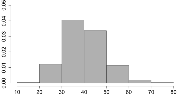
Relative frequency density histograms display the distribution of data. For large data sets, changing the width of the intervals will typically not change the overall shape of the histogram but rather reveal details of the distribution. Decreasing the interval width is like increasing the resolution of a picture.
The area of the rectangles over a collection of intervals represents the proportion of data that falls into these intervals. In particular, the total area of a relative frequency density histogram is always 1.
Imagine that you have an extremely large data set and you decrease the intervals to a very small width. In this case you might find that the shape of the resulting histogram can be approximated by a smooth curve.
Click on the histogram below to decrease the width of the intervals.
Since the total area of the histogram is 1, the area under the curve also has to be 1. This leads to the concept of a density curve.
A density curve is a curve on or above the horizontal axis such that the area between the horizontal axis and the curve is 1.
Just as data have a mean and a standard deviation, one can define mean and standard deviation for density curves. The precise definitions of these terms require some calculus and therefore cannot be given in this algebra-based statistics course. Intuitively, however, the mean and the standard deviation of a density curve are approximately the mean and the standard deviation of a very large data set whose relative frequency density histogram can be approximated by the density curve. The mean of a density curve is denoted by \(\mu\) and the standard deviation is denoted by \(\sigma . \)
| The mean \(\mu\) of a density curve can be visualized as the location where the area under the density curve, if it were made from some solid material, would balance. | 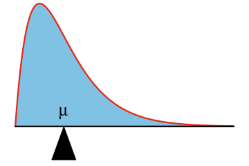
|
One can define all the other measures of center and measures of spread for density curves. The median for example is the value on the horizontal axis such that the area to its left under the density curve is 0.5.
For a symmetric density curve the mean and the median are always the same.
What is the distribution of the weights of babies at birth? What is the distribution of the heights of female or male students at Auburn University? What is the distribution of body temperature among adults?
If you collected data for any of these variables (weight, height, body temperature), you would find that the histograms of these data are mound shaped and could be approximated by a certain density curve.
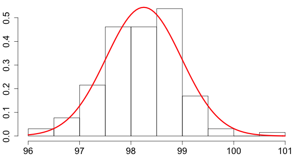
The graph below is a histogram of data consisting of body temperatures measured in Fahrenheit of 130 subjects which is overlaid by a so-called normal density curve, which is the density curve of a normal distribution.
The density curve for a normal distribution is not just any mound shaped or bell shaped curve. It can be described by an equation that contains two parameters, \(\mu\) (read: mu) and \(\sigma\) (read: sigma). More precisely, the curve is the graph of the equation \(y=f(x),\) where \[ f(x) = \frac{1}{\sqrt{2\pi \sigma^2}}\exp \left( \frac{-(x-\mu)^2}{2\sigma^2}\right), \] \(\mu\) can be any number, and \(\sigma\) any positive number.
Different values for \(\mu\) and \(\sigma\) will yield different density curves. Change the values of these parameters by dragging the sliders in the graph below and observe how the density curve changes.
Note that the parameter \(\mu\) is located at the peak and the parameter \(\sigma\) describes the width of the density curve.
| The normal density curve bends downward in the center and bends upward further away from the center. There are two points on the curve that separate bending upward from bending downward. The standard deviation turns out to be half the distance between these 2 points. |  |
Suppose we have many measurements of body temperature of adult male humans and the distribution of the data is approximately normal with mean \(\mu=36.7\) Celsius and standard deviation \(\sigma = 0.4\) Celsius. For brevity, denote the variable that describes body temperature by \(X.\) Then we write \(X \sim N(\mu=36.7, \sigma=0.4)\) (read: \(X\) is normally distributed with parameters \(\mu=36.7\) and \(\sigma=0.4.\))
Here are some typical questions.
To answer these questions we need the function \(F,\) where \(F(x)\) is equal to the area to the left of \(x\) under the normal density curve, and the function \(G,\) where \(G\) is the inverse of \(F.\) Since there is no simple formula for \(F\) or \(G,\) the most convenient way to solve these questions is to use a software package where these functions are available.
In the statistical software package R these two functions are called pnorm() and qnorm().
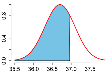
1. What proportion of the measurements is less than 37.1 Celsius?
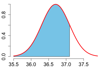 |
The shaded area is 0.8413447. It is calculated with:
|
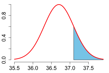
2. What proportion of the measurements is greater than 37.1 Celsius?
|
The shaded area is 0.1586553. It is calculated with:
|
3. What proportion of the measurements is between 36.3 and 37.1 Celsius?
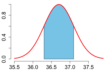 |
The shaded area is 0.6826895. It is calculated with:
|
4. Find the lower quartile of the data? In other words, find a number \(x\) such that the area under the density curve left of \(x\) is 0.25.
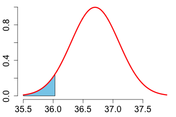 |
The 0.25 quantile is 36.4302 Celsius. It is calculated with:
|
5. Find the value \(x\) such that 95 percent of the data is at most \(x.\)
 |
The 0.95 quantile is 37.35794 Celsius. It is calculated with:
|
So far we've considered the distribution of measurements of a variable \(X\), where \(X\sim N(\mu=36.7, \sigma=0.4).\) How would the distribution change if we multiplied each value of \(X\) by a constant value, say \(a\)?
In this case the distribution of \(Y=aX\) would also be normal but the parameters would be scaled by \(a\), that is, \(Y \sim N(\mu=a\cdot 36.7, \sigma=a\cdot 0.4). \)
How would the distribution change if we added a constant value, say \(b\), to each measurement of \(X\)?
In this case the distribution of \(Y=X+b\) would have the same shape as the distribution of \(X\) but it would be shifted by \(b\) units to the right. That is, \(Y \sim N(\mu=36.7+b, \sigma=0.4). \)
In general, if \(X \sim N(\mu_X, \sigma_X)\), \(a\) and \(b\) are constants, \(b\neq 0\), \(Y=aX+b\), then \(Y \sim N(\mu_Y, \sigma_Y), \) where \(\mu_Y=a \mu_X+b\) and \(\sigma_Y=|a|\sigma_X. \)
Here is an application for this transformation rule. Suppose you want to report the results for body temperatures in Fahrenheit rather than in Celsius. In this case, a measurement of \(X\) in Celsius is transformed to the measurement \(Y=\frac{9}{5}X+32\) in Fahrenheit. Since \(X\sim N(\mu_X=36.7, \sigma_X=0.4)\) it follows from the transformation rule that \(Y\sim N(\mu_Y = 98.06, \sigma_Y = 0.72)\).
The proportion of measurements of \(X\) less than 37.1 is then equal to the proportion of measurements of \(Y\) less than \(\frac{9}{5}37.1+32 = 98.78.\)
The transformation rule allows us to transform problems of the type considered above to a problem with particular parameters. Therefore we only need the functions \(F\) and \(G\) for a particular normal distribution and if you didn't have a calculator or computer then only one table would be needed. Tables were necessary before computers and appropriate software were available. Using tables requires more work and errors are more likely.
Since it is easy to transform to and from the distribution \(N(\mu=0, \sigma=1)\), it would be best to create a table for this distribution. Let's call this distribution the standard normal distribution.
If in some application the measurements of a variable \(X\) are \(N(\mu, \sigma)\) then we could transform each measurement \(x\) to the value \[ z=\frac{x-\mu}{\sigma}. \]
Let's call this value the standardized value of \(x\) or the z-score of \(x\). Then any question we have about the measurements of \(X\) can be formulated as a question about the standardized values.
The z-score is a measure of relative standing. It tells you how many standard deviations the value \(x\) is above or below the mean \(\mu .\) It is most useful when the distribution of the data is approximately normal because in that case we can convert it to a percentile. With some practice you can look at a z-score of x and have a good sense of the relative position of \(x\) to the rest of the data. The following rule helps in developing this sense. Memorize it!
Empirical Rule (also called the 68-95-99.7 Rule). Suppose that measurements of the variable \(X\) are approximately normally distributed. Then approximately
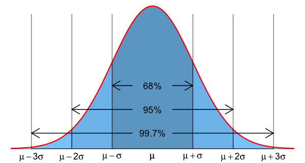
Here is an application of the Empirical Rule. Suppose that body temperatures for adult men are normally distributed with a mean of 36.7 Celsius and a standard deviation of 0.4 Celsius. Bob's temperature is 37.6 Celsius. The z-score of this temperature is 2.25. According to the Empirical Rule, 95% of body temperatures are within 2 standard deviations of the mean. Bob's temperature is more than two standard deviations above the mean. Since only 5% of body temperatures are more than 2 standard deviations away from the mean, by symmetry, only 2.5% are more than 2 standard deviations above the mean. We conclude that less than 2.5% have a temperature as high as Bob's. Since this is unusual, Bob might have a fever.
The 68-95-99.7 rule only applies for data that is approximately normally distributed. How do we check if this is the case? How do we know that measurements of a given variable \(X\) have a normal distribution?
We could plot a histogram of the data and inspect its shape. But there is a better way. In order to explain that better way I need to tell you about quantiles for a density curve.
For a number p, \(0\lt p \lt 1\), the p quantile is the number q such that the area to the left of q under the density curve is p.
For example, if \(p=0.95\) then the 0.95-quantile for the distribution \(N(\mu=36.7, \sigma=0.4)\) is the value \(q=37.4\) (rounded). Instead of calling 37.4 the 0.95-quantile we can also call it the 95th percentile. The p-quantile is the same as the 100p-th percentile.
Without knowing it, we have been calculating quantiles in some of the previous problems. We just need the function \(G,\) which is the inverse of the function \(F,\) to calculate quantiles. Also note that the quartiles and the median are just special cases of quantiles.
While there is no standard definition of quantiles for data, the quantiles for the density curve of a normal distribution are well defined. For \(p\), \(0\lt p \lt 1\), there is exactly one point \(q\) such that the area to the left of \(q\) is \(p\).
What happens when you plot the quantiles of a normal distribution against the same quantiles of another normal distribution? Let's say you plot the 0.1, 0.2, 0.3, and 0.7 quantiles of the distribution \(N(\mu=36.7, \sigma=0.4)\) against the 0.1, 0.2, 0.3 and 0.7 quantiles of the distribution \(N(\mu=0, \sigma=1)\).
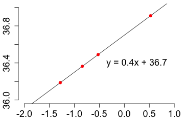 |
All the points lie on a straight line! Note that the slope and the intercept of the line are given by \(\sigma\) and \(\mu\) of the distribution \(N(36.7, 0.4). \) |
Suppose that you wanted to know if the measurements of a variable \(X\) have a normal distribution. You could use the measurements of \(X\) to estimate certain quantiles of the distribution of \(X\). Then you could plot these estimated quantiles against the corresponding quantiles of the standard normal distribution. If the distribution of \(X\) is approximately normal then all the points should be close to a straight line. Since we are plotting estimated quantiles against exact quantiles, we call this a quantile-quantile plot or simply Q-Q plot.
Here is the Q-Q plot of 130 measurements of body temperature. Overall, the plot has a straight line pattern. The point in the upper right corner is an outlier and should be investigated.

If the plot does not follow a straight line, then the data's having a normal distribution becomes dubious.
Suppose \(X \sim N(\mu=36.7, \sigma=0.4).\) Then the area to the left of 38 is calculated with the function pnorm().
| pnorm(38, mean=36.7, sd=0.4) |
If some data is approximately normally distributed with parameters \(\mu = 36.7\) and \(\sigma = 0.4\) then the area to the left of 38 is interpreted as the proportion of data that is at most 38.
Since the total area under the density curve is always 1, the area to the right of 38 is found as follows.
| 1-pnorm(38, mean=36.7, sd=0.4) |
To find a particular quantile or percentile for the density curve of \(X\) the function qnorm() is used. For example, the 0.9 quantile or 90th percentile is found as follows.
| qnorm(0.9, mean=36.7, sd=0.4) |
Suppose the values of a variable are stored in the variable \(x\) in R. Then the normal Q-Q plot of the values stored in \(x\) is calculated with the function qqnorm().
| x = c(36.7, 36.6, 36.8, 37.0, 37.2, 36.8, 37.2, 36.6, 36.7, 36.4) |
| qqnorm(x) |