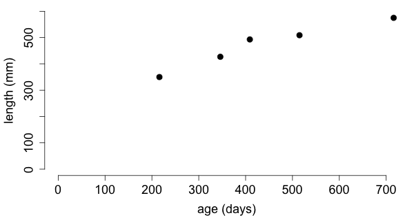
What is the relationship between age and length of a Western Hognose Snake (Heterodon nasicus)?
| date | age (x) | length (y) |
|---|---|---|
| 2/16/08 | 216 days | 350 mm |
| 5/25/08 | 346 days | 427 mm |
| 8/27/08 | 409 days | 493 mm |
| 12/11/08 | 515 days | 509 mm |
| 5/30/09 | 716 days | 575 mm |
Data provided by Gerda M. Zinner.
The scatterplot reveals a strong linear relationship between age
and length.
Since there appears to be a linear relationship between the two variables it would be reasonable to describe the relationship with a straight line.
Move the straight line on the scatterplot by dragging the points A and B until you achieve a good fit of the line to the data.
There may be nothing wrong with the line that you created but it would be better to have a procedure for drawing the line so that everyone gets the same line. In addition we would like to draw the line that has the best fit to the data.
How do we decide if one line fits better than another line?
We need to find a way to measure how well a line fits the data. There are many ways to do this. Here is one:
Take the vertical distance of each point to the line, square it, and add all of them together. The smaller the sum of squares, the better the fit.
Minimize the sum of squares, which is the area of all the squares, by adjusting the line in the scatterplot below.
Using calculus or linear algebra, one can derive a formula for the line that minimizes the sum of squares: \[ \hat y = b_0 + b_1 x \quad \mbox{where} \quad b_1=r\frac{s_y}{s_x}, \quad b_0=\bar y - b_1 \bar x, \] \(r\) denotes the correlation coefficent of the two variables, \(s_x\) and \(s_y\) are the sample standard deviations of \(x\) and \(y, \) and \(\bar x\) and \(\bar y\) are the sample means of \(x\) and \(y .\) This line is called the least squares regression line.
Calculating the least squares regression line is best done with appropriate software. Using R we find that the equation of the least squares regression line is given by: \[ \hat y = 277.85591 + 0.43811 x \]
Why does it help to have the equation for the least squares regression line?
The equation for the least squares regression line can be used for predicting the response \(y\) to a given value of \(x.\) That is why this equation is also called the prediction equation.
What was the length of the snake when it was 600 days old?
| The predicted value of the length \(y\) for the age \(x = 600\) is \[ \begin{eqnarray*} \hat y & = & 277.85591 + 0.43811 \times 600 \\ & = & 540.7219. \end{eqnarray*} \] |  |
Typically we don't know if the linear pattern persists outside the range of the collected data, and therefore one should not make predictions in such a case. In fact, in our example one would expect that the growth of the snake will eventually slow down.
Note that for \(x=0,\) \(\hat y = b_0 + b_1 x = b_0\), that is, the intercept \(b_0\) is the predicted response when the explanatory variable \(x\) is 0.
In our example, the intercept is the length of the snake at birth. Since we don't know whether or not there is a linear relation between age and length beyond the measured range, this interpretation is not valid.
The slope can always be interpreted as the change in the response for a unit change in the explanatory variable.
If the run(change in \(x\)) is 1, then the rise(change in \(y\)) is equal to the slope of the line. |
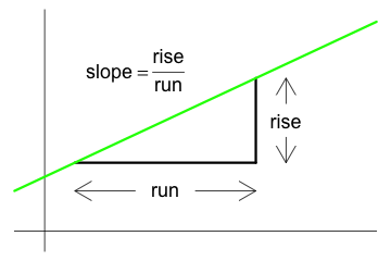 |
During a single day, the length of the snake increases by about \(b_1=0.44\) mm. Equivalently, in two months the snake grows by about 1 inch.
Note that the slope \(b_1\) and the correlation coefficient \(r\) are related by the formula \(b_1 = r\frac{s_y}{s_x}\) and that the predicted value for \(x=\bar x\) is \(y=\bar y. \) It follows that \[ \frac{\hat y - \bar y}{x -\bar x} = r\frac{s_y}{s_x} \] and therefore \[ \frac{\hat y - \bar y}{s_y} = r\frac{x -\bar x}{s_x} . \] Since \(r\) is less than 1, unless all the points lie on a straight line, the \(z\)-score of the predicted value of \(y\) is less than the \(z\)-score of \(x\) in absolute values. In other words, measuring distances in terms of standard deviations, the predicted value of \(y\) is closer to the mean \(\bar y\) than the value \(x\) is to its mean \(\bar x .\)
This effect was noted first by Sir Francis Galton in the late 1800s when he studied the relationship between the heights of fathers and sons. Suppose for the sake of simplicity that the standard deviations and average heights of fathers and sons are the same. Then the son of a tall father is likely to be tall but not quite as tall as the father. The son of a short father will be short but not quite as short as the father. Galton described this effect as regression to the mean
and from that expression evolved the phrase least squares regression line.
| A point in the scatterplot that is far away from all the other points, is called an outlier. The points labeled A and B are both outliers. | 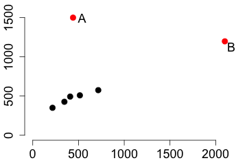 |
An observation that would substantially change the prediction equation if it were removed is called an influential observation. An influential observation is typically an outlier, but an outlier may or may not be an influential observation.
Move the outlier, point B, around and observe how the regression line changes. The dashed line is the regression line without the outlier. Point B is not influential when the dashed and the solid lines are close to each other.
While one can detect outliers and influential observations from a scatterplot, it is easier to find them in a so-called residual plot. The residuals are the observed values of \(y\) minus the predicted values of \(y\); they are the vertical deviations of the data to the regression line. A residual plot is a scatterplot of the residuals against the values of the explanatory variable.

The vertical lines are not usually drawn in a residual plot. They are plotted here only to emphasize that the residuals are the vertical deviations from the regression line.
Detecting influential observations is more difficult than detecting outliers. One has to remove the suspected observations to see whether the answers to the relevant questions change.
There is no good interpretation of the correlation coefficient \(r.\) We distinguish between strong, moderate and weak correlation somewhat arbitrarily. It turns out that the square of \(r\) can be more readily interpreted in the context of linear regression.
One can show that \[ r^2 = 1-\frac{\sum{(y_i-\hat y_i)^2}}{\sum{(y_i - \bar y)^2}}. \]
Since \(\sum{(y_i - \bar y)^2}\) is a measure for the variation in the variable \(y\) and \(\sum{(y_i-\hat y_i)^2}\) is a measure for the variation in the residuals of \(y\), the fraction \(\frac{\sum{(y_i-\hat y_i)^2}}{\sum{(y_i - \bar y)^2}}\) is interpreted as the proportion of variation in \(y\) that is not explained by the linear regression.
The coefficient of determination \(r^2\) is interpreted as the proportion of the variation in the response variable that is explained by the explanatory variable using a linear regression model.
In our example, \(r^2 = 0.9281\) is interpreted to mean that 93 percent of the variation in the length of the snake is explained by the age of the snake in a linear regression model.
The least squares regression line for the data given above can then be calculated with the function lm() (lm
stands for linear model).
| x = c(216, 346, 409, 515, 716) |
| y = c(350, 427, 493, 509, 575) |
| lm(y~x) |
One way to add the least squares regression line to the scatterplot is to first store the fitted model calculated with lm() in a variable, say fm and then use the function abline().
| plot(x,y) |
| fm = lm(y~x) |
| abline(fm) |
If the linear regression model is stored in the variable fm, then the residuals can be calculated with the function residuals() and the residual plot is created as follows.
| plot(x, residuals(fm)) |
The coefficient of determination is just the square of the correlation coefficient.
| cor(x, y)^2 |
You can predict the values of y for certain values of x, say \(x=600\) and \(x=800\) using the following method.
| new = data.frame(x=c(600, 800)) |
| predict(fm, new) |
Note that predicting y for a value of x that is outside the range of collected data is usually not appropriate because the observed linear pattern may not extend to this range.