Matrix multiplication

Lecture 4

Author

Affiliation

Minjae Park

Auburn University
MATH 2660 - Spring 2026

Recap

$$ % Colors

% Coordinate vectors and matrices

% Common sets

% Abstract vector symbols

% Norms / absolute value

% Optional: dot product spacing (looks nicer in slides)

% Operators $$

Linear combinations and matrix notation

• An \(n\times k\) matrix represents \(k\) vectors in \(\mathbb{R}^n\).
• Each vector forms a column of the matrix: \[ \begin{bmatrix} \boxed{\begin{array}{c} v_{11} \\ \vdots \\ v_{n1} \end{array}} & \boxed{\begin{array}{c} v_{12} \\ \vdots \\ v_{n2} \end{array}} & \cdots & \boxed{\begin{array}{c} v_{1k} \\ \vdots \\ v_{nk} \end{array}} \end{bmatrix} \]
• We write this compactly as \([\vec{v}_1\ \vec{v}_2\ \cdots\ \vec{v}_k\)] (block notation).

• A linear combination of vectors \(\vec{v}_1,\dots,\vec{v}_k\) is a vector of the form \[ \vec{u} = c_1\vec{v}_1 + \cdots + c_k\vec{v}_k = \sum_{i=1}^k c_i\vec{v}_i, \] where the coefficients \(c_i\in\mathbb{R}\).
• If we encode the vectors into a matrix \(A=[\vec{v}_1\ \cdots\ \vec{v}_k]\) and the coefficients into a vector \[ \vec{c} = \begin{bmatrix} c_1 \\ \vdots \\ c_k \end{bmatrix}, \] then the linear combination can be written as a matrix multiplication \[ \vec{u} = A\vec{c}. \]

Get familiar with notational convention

\[ \begin{bmatrix} v_{\boxed{\phantom{\;\;}}} & v_{\boxed{\phantom{\;\;}}} & \cdots & v_{\boxed{\phantom{\;\;}}} \\ v_{\boxed{\phantom{\;\;}}} & v_{\boxed{\phantom{\;\;}}} & \cdots & v_{\boxed{\phantom{\;\;}}} \\ \vdots & \vdots & \ddots & \vdots \\ v_{\boxed{\phantom{\;\;}}} & v_{\boxed{\phantom{\;\;}}} & \cdots & v_{\boxed{\phantom{\;\;}}} \end{bmatrix} \begin{bmatrix} c_{\boxed{\phantom{\;\;}}} \\ c_{\boxed{\phantom{\;\;}}} \\ \vdots \\ c_{\boxed{\phantom{\;\;}}} \end{bmatrix} \\ = \begin{bmatrix} c_{\boxed{\phantom{\;\;}}}v_{\boxed{\phantom{\;\;}}} + c_{\boxed{\phantom{\;\;}}}v_{\boxed{\phantom{\;\;}}} + \cdots + c_{\boxed{\phantom{\;\;}}}v_{\boxed{\phantom{\;\;}}} \\ c_{\boxed{\phantom{\;\;}}}v_{\boxed{\phantom{\;\;}}} + c_{\boxed{\phantom{\;\;}}}v_{\boxed{\phantom{\;\;}}} + \cdots + c_{\boxed{\phantom{\;\;}}}v_{\boxed{\phantom{\;\;}}} \\ \vdots \\ c_{\boxed{\phantom{\;\;}}}v_{\boxed{\phantom{\;\;}}} + c_{\boxed{\phantom{\;\;}}}v_{\boxed{\phantom{\;\;}}} + \cdots + c_{\boxed{\phantom{\;\;}}}v_{\boxed{\phantom{\;\;}}} \end{bmatrix}. \]

Fill these in by using your conceptual understanding of matrix notation and matrix multiplication. (Hint: what is the meaning of column blocks? What is the meaning of \(v_{ij}\)?)

Matrix Multiplications

Coordinate system revisited

• In the Cartesian coordinate system, the coordinates \((3,-2)\) is interpreted as: “move 3 units in the \(\vec e_1\) direction, then move \(-2\) units in the \(\vec e_2\) direction.”
• What if we use a different coordinate system, with axes \[ \vec v_1 = \langle -1,0 \rangle, \qquad \vec v_2 = \langle 1,1 \rangle? \]
• Can you relate this to a linear combination?
• How can we visualize this movement?

Two coordinates of the same movement

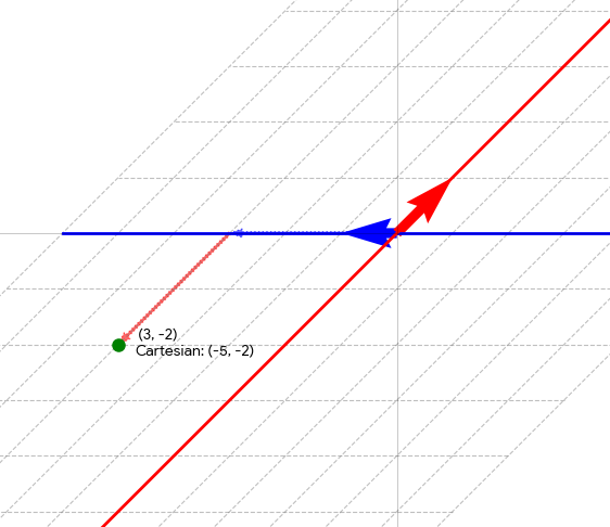
Coordinate change

• We agree on the movement of \((3,-2)\) only after specifying a coordinate system.
• The movement is intrinsic, but its coordinate representation depends on the chosen system.
• When we write \[ \vec v_1 = \langle -1,0 \rangle, \qquad \vec v_2 = \langle 1,1 \rangle, \] these vectors are given in the Cartesian coordinate system.
• Once this information is known, we can convert coordinates from a new coordinate system into Cartesian coordinates.
• Matrix multiplication is exactly the tool that performs this conversion.

Matrix and coordinate change

• Interpret \(A = [\vec v_1 \ \vec v_2 \ \cdots \ \vec v_k]\) as the matrix encoding the axes of a new coordinate system (expressed in the Cartesian system).
• Let \(\vec u = \langle u_1,\dots,u_k \rangle\) be the coordinates of a point in this new system.
• Then \[\vec w = A\vec u\] gives the Cartesian coordinates of that point.

Coordinate change for multiple points

• In a fixed coordinate system, the axes stay the same, while different coordinates represent different points.
• Often, we want to convert many points at once from a new coordinate system into Cartesian coordinates.
• This can be done by placing multiple coordinate vectors side by side.

Matrix multiplication

Suppose we have \(m\) coordinate vectors \(\vec c_1,\dots,\vec c_m\). We collect them into a matrix: \[ [\vec c_1 \ \vec c_2 \ \cdots \ \vec c_m] = \begin{bmatrix} c_{11} & c_{12} & \cdots & c_{1m} \\ c_{21} & c_{22} & \cdots & c_{2m} \\ \vdots & \vdots & \ddots & \vdots \\ c_{k1} & c_{k2} & \cdots & c_{km} \end{bmatrix}. \]

In the new coordinate system, the axes \(\vec v_1,\dots,\vec v_k\) are encoded by \[ [\vec v_1 \ \vec v_2 \ \cdots \ \vec v_k] = \begin{bmatrix} v_{11} & v_{12} & \cdots & v_{1k} \\ v_{21} & v_{22} & \cdots & v_{2k} \\ \vdots & \vdots & \ddots & \vdots \\ v_{n1} & v_{n2} & \cdots & v_{nk} \end{bmatrix}. \]

Matrix multiplication (block notation)

• We define \[ [\vec v_1 \ \cdots \ \vec v_k] [\vec c_1 \ \cdots \ \vec c_m] = [\vec w_1 \ \cdots \ \vec w_m], \] where each column satisfies \[ [\vec v_1 \ \cdots \ \vec v_k]\vec c_\ell = \vec w_\ell. \]

Matrix multiplication (full expansion)

\[ \begin{bmatrix} v_{11} & v_{12} & \cdots & v_{1k} \\ v_{21} & v_{22} & \cdots & v_{2k} \\ \vdots & \vdots & \ddots & \vdots \\ v_{n1} & v_{n2} & \cdots & v_{nk} \end{bmatrix} \begin{bmatrix} c_{11} & c_{12} & \cdots & c_{1m} \\ c_{21} & c_{22} & \cdots & c_{2m} \\ \vdots & \vdots & \ddots & \vdots \\ c_{k1} & c_{k2} & \cdots & c_{km} \end{bmatrix} \\ = \begin{bmatrix} w_{11} & w_{12} & \cdots & w_{1m} \\ w_{21} & w_{22} & \cdots & w_{2m} \\ \vdots & \vdots & \ddots & \vdots \\ w_{n1} & w_{n2} & \cdots & w_{nm} \end{bmatrix}. \] with \(w_{i\ell} = c_{1\ell}v_{i1} + c_{2\ell}v_{i2} + \cdots + c_{k\ell}v_{ik} = w_{i\ell} = \sum_{j=1}^k c_{j\ell}\, v_{ij}.\)

• This is the general matrix multiplication, extending the earlier case of multiplying a matrix by a single vector.
• Interpretation of each matrix:
  • \(n\times k\): axes of the new coordinate system
    
  • \(k\times m\): coordinates of \(m\) points in that system
    
  • \(n\times m\): Cartesian coordinates of the same points

• Dimension check: \((n\times k)\cdot(k\times m) \Rightarrow (n\times m)\), so matrix multiplication is defined precisely when the middle dimensions match.
• Interpretation:
  • if you have \(k\) axes, then each point must be described using \(k\) coordinates.
  • Since each axis is a vector in \(\mathbb{R}^n\), multiplying by \(m\) such coordinate vectors produces \(m\) Cartesian points in \(\mathbb{R}^n\).

Example

• Consider the coordinate system with two axes \[ \vec v_1=\langle -1,0 \rangle, \qquad \vec v_2=\langle 1,1 \rangle. \]
• In this system, consider four points with coordinates \[ (3,-2), \quad (0,1), \quad (2,0), \quad (1,1) \]
• Use one matrix multiplication to find the Cartesian coordinates of all four points.
• Type your answer in the form \((x_1,y_1), (x_2, y_2), (x_3,y_3), (x_4,y_4)\).

Scan the QR code or go to join.iclicker.com/MBNJ.

Note: If you are completely lost, or facing any difficulties, please briefly explain your situation instead.

Computer-aided calculations

• Many exercises in this course are designed to build your eyeball and muscle memory for new concepts, rather than to practice perfectly error-free calculations.
• In practice, computers and calculators are often more reliable than humans, and knowing how to use them effectively is an important skill.
• For the best learning experience, I recommend first working through exercises by hand to develop understanding (which is much more effective than simply reading worked-out solutions), and then checking your results using a computer.

MATLAB

• One widely used computational tool in engineering and applied sciences is MATLAB.

• You may install MATLAB on your laptop, or use the web version on any device.

• Try typing the following command:

    [-1 1; 0 1] * [3 0 2 1; -2 1 0 1]