Least squares approximations

Lecture 18

Minjae Park

Auburn University
MATH 2660 - Spring 2026

February 20, 2026

Attendance

Scan the QR code or go to join.iclicker.com/MBNJ.

In many real-world applications, we want to solve \(A\vec{x}=\vec{b}\), where \(A\) is determined from a mathematical model and \(\vec{b}\) is obtained from experimental or observed data.
However, the model may not be perfect and the data may contain noise, so the system \(A\vec{x}=\vec{b}\) may have no exact solution.
In this case, we try to find the best possible \(\vec{x}\) by making \(A\vec{x}\) as close to \(\vec{b}\) as possible.
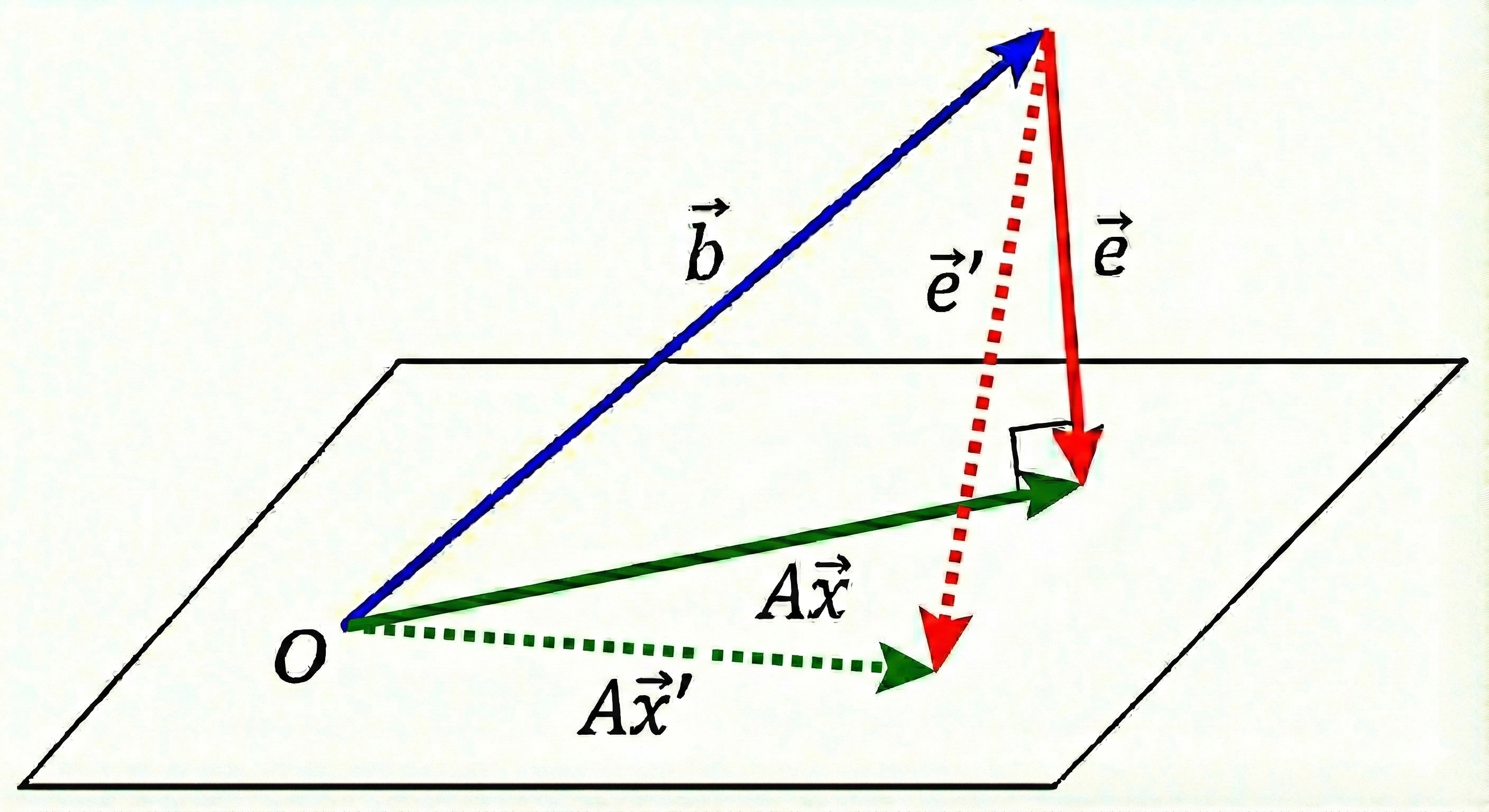
Define the error vector \(\vec{e} = A\vec{x} - \vec{b}\).
To measure “closeness,” we minimize the length (Euclidean norm) of the error: \[\left\lVert \vec{e} \right\rVert = \sqrt{\vec{e} \!\cdot\!\vec{e}}.\]

Goal: find \(\vec{x}\) such that \(A\vec{x}\) is closest to \(\vec{b}\).
Geometric intuition: the vectors \(A\vec{x}\) form a subspace \[W = \text{span}\{\vec{u}_1,\dots,\vec{u}_n\},\] where \(\vec{u}_i\) are the columns of \(A\).
In general, \(\vec{b} \notin W\), so \(A\vec{x}=\vec{b}\) has no solution.
The best approximation occurs when we project \(\vec{b}\) orthogonally onto \(W\).
Thus, the least squares solution corresponds to the orthogonal projection of \(\vec{b}\) onto \(W\).

Let \(A = [\vec{u}_1 \ \dots \ \vec{u}_n]\).
Recall: \[A^T\vec{v} = \begin{bmatrix} \vec{u}_1 \!\cdot\!\vec{v} \\ \vdots \\ \vec{u}_n \!\cdot\!\vec{v} \end{bmatrix}.\]
If \(\vec{v}\) is orthogonal to every column \(\vec{u}_i\), then \(A^T\vec{v}=\vec{0}\). In this case, \(\vec{v}\) is orthogonal to the entire subspace \(W = \text{span}\{\vec{u}_1,\dots,\vec{u}_n\}\).
Thus, for the best approximation, the error \(\vec{e} = A\vec{x}-\vec{b}\) must satisfy \[A^T\vec{e} = 0.\]

Therefore, \[A^T(A\vec{x}-\vec{b})=0,\] which gives the normal equations \[A^TA\vec{x} = A^T\vec{b}.\]
Geometrically, this system always has a solution (when columns of \(A\) are linearly independent).

Let \[ A=\begin{bmatrix} 1 & 2 \\ 1 & \tfrac{3}{2} \\ 1 & 4 \end{bmatrix}, \qquad \vec{b}=\begin{bmatrix}1\\2\\1\end{bmatrix}. \]

Describe in words the geometric meaning of the least squares approximation to \(A\vec{x} \approx \vec{b}\).
Compute the best approximation \(\vec{x}\) by solving the normal equations.

The table shows the world population (in billions) for six different years (Source: U.S. Census Bureau).

Year	1985	1990	1995	2000	2005	2010
Population	4.9	5.3	5.7	6.1	6.5	6.9

Let \(x=5\) represent the year 1985 (so \(x=10\) is 1990, etc.).

The table shows the mean distances \(x\) (in astronomical units) and orbital periods \(y\) (in years) of six planets closest to the Sun.

Planet	Mercury	Venus	Earth	Mars	Jupiter	Saturn
Distance \(x\)	0.387	0.723	1.000	1.524	5.203	9.537
Period \(y\)	0.241	0.615	1.000	1.881	11.862	29.457

We expect a power model of the form \(y = Cx^k\).
Take logarithms: \(\ln y = \ln C + k \ln x\).
This becomes a linear regression problem in variables \(Y=\ln y, \quad X=\ln x\).
Use least squares to determine \(\ln C\) and \(k\).
Result relates to Kepler’s Third Law: \(y^2 \propto x^3\).

In signal processing, it is useful to decompose a signal into different frequency components.
Let \(f:[0,2\pi]\to\mathbb R\) be continuous.
A Fourier series representation is \[ f(x)=\frac{a_0}{2}+\sum_{n=1}^{\infty}\big(a_n\cos(nx)+b_n\sin(nx)\big). \]
Interpretation:
- \(f\) is written as a linear combination of \(\{1,\cos x,\cos 2x,\dots,\sin x,\sin 2x,\dots\}\).
- Each \(\cos(nx)\) and \(\sin(nx)\) represents the \(n\)th frequency mode.
- The coefficients \(a_n,b_n\) represent amplitudes.

Consider the inner product on \(C([0,2\pi])\): \[\left\langle f,g \right\rangle=\int_0^{2\pi} f(x)g(x)\,dx.\]
Orthogonality relations: \[ \int_0^{2\pi}\cos(ix)\cos(jx)\,dx= \begin{cases} \pi & i=j\neq0 \\ 2\pi & i=j=0 \\ 0 & i\ne j \end{cases} \] \[ \int_0^{2\pi}\sin(ix)\sin(jx)\,dx= \begin{cases} \pi & i=j \\ 0 & i\ne j \end{cases} \] \[ \int_0^{2\pi}\cos(ix)\sin(jx)\,dx=0 \quad \text{for all } i,j. \]

Theorem: any continuous function can be represented uniquely by its Fourier series.
After normalization, the set \[ S=\left\{\frac{1}{\sqrt{2\pi}},\frac{\cos(nx)}{\sqrt{\pi}},\frac{\sin(nx)}{\sqrt{\pi}}:n\ge1\right\} \] is an orthonormal basis of \(C([0,2\pi])\).

A musical sound wave is a superposition of many different frequencies produced by instruments and voices. 🎥Visualization
Each frequency band corresponds to a certain instrument, tone color, or vocal range (bass, mid, treble).
Using a Fourier decomposition, the sound signal can be written as a sum of frequency modes with different amplitudes.
An equalizer adjusts the amplitudes of selected frequency modes to enhance or suppress certain components.
For example, we can boost low frequencies (bass), reduce harsh high frequencies, or emphasize vocal ranges.
The same idea is used in noise-canceling: suppress unwanted frequency bands (e.g., airplane engine noise) while preserving or amplifying human speech.

A digital image can also be viewed as a “signal,” where the pixel values represent function values.
Smooth regions in an image correspond to low-frequency components, while rapid changes in intensity correspond to high-frequency components.
By enhancing high-frequency components, we can make edges more visible (edge detection).
By suppressing high-frequency components, we can smooth the image (blur or noise reduction).
Early image-processing tools (including older Photoshop techniques such as skin retouching) relied on this frequency separation idea.
📰 What are Filtering in Frequency Domain and Fourier Transform?

Recall \(f(x)=\frac{a_0}{2}+\sum_{n=1}^{\infty}\big(a_n\cos(nx)+b_n\sin(nx)\big)\).
Using orthogonality: \[ a_n=\left\langle f,\frac{1}{\pi}\cos(nx) \right\rangle = \frac{1}{\pi}\int_0^{2\pi} f(x)\cos(nx)\,dx,\quad n\ge1, \] \[ b_n=\left\langle f,\frac{1}{\pi}\sin(nx) \right\rangle = \frac{1}{\pi}\int_0^{2\pi} f(x)\sin(nx)\,dx,\quad n\ge1, \] \[ a_0=2\left\langle f,\frac{1}{2\pi} \right\rangle = \frac{1}{\pi}\int_0^{2\pi} f(x)\,dx. \]
These are called the Fourier coefficients.

In practice, we cannot compute or store infinitely many Fourier coefficients.
Fortunately, most of the essential (global) features of a function are captured by low-frequency modes, while high-frequency modes often encode fine details or noise.
We approximate \(f\) by truncating its Fourier series: \[ f(x)\approx \frac{a_0}{2}+\sum_{n=1}^{N}\big(a_n\cos(nx)+b_n\sin(nx)\big). \]
This truncated series is the orthogonal projection of \(f\) onto the finite-dimensional subspace \[ \text{span}\{1,\cos x,\dots,\cos(Nx),\sin x,\dots,\sin(Nx)\}. \]

In many real-world applications, mathematical models are imperfect because we ignore noise or cannot include all possible parameters.
When fitting parameters in a regression problem \(A\vec{x} \approx \vec{b}\), we use least squares approximation, which minimizes the size of the error vector.
The least squares solution satisfies the normal equations \[ A^TA\vec{x} = A^T\vec{b}. \]
Fourier approximation is a special case of least squares approximation, where the “size” of the error is measured using an inner product for functions.
In particular, a truncated Fourier series is the orthogonal projection of a continuous function onto the vector space spanned by low-frequency trigonometric basis functions.