Applications of determinants

Lecture 25

Minjae Park

Auburn University
MATH 2660 - Spring 2026

March 18, 2026

Attendance

Scan the QR code or go to join.iclicker.com/MBNJ.

Recap

Determinants

For an \(n\times n\) matrix \(A\):
- \(\det(A)\) can be computed by cofactor expansion along any row or column; in practice, choose one with many zeros to simplify the computation.
- \(|\det(A)|\) equals the hypervolume of the parallelepiped spanned by the \(n\) column vectors of \(A\).
- The sign of \(\det(A)\) records the orientation of the column vectors.
- If \(\det(A)=0\), the columns are linearly dependent.
- If \(\det(A)\neq0\), the columns are linearly independent and \(A\) is invertible.

Properties of Determinants

For \(n\times n\) matrices \(A\) and \(B\), \[ \det(AB)=\det(A)\det(B), \] and therefore \(\det(AB)=\det(BA)\).
\(A\) is invertible if and only if \(\det(A)\neq0\); in that case, \[ \det(A^{-1})=\frac{1}{\det(A)}. \]
Determinants of elementary matrices are easy to compute, so \(\det(A)\) can be computed efficiently using Gaussian or Gauss–Jordan elimination.
(*) The determinant is invariant under transpose: \(\det(A^T)=\det(A)\).

Matrix Transposes Revisited

Transpose of Multiplication

Let \(A=[\vec{u}_1\ \dots\ \vec{u}_n]\) be a \(k\times n\) matrix and \(B=[\vec{v}_1\ \dots\ \vec{v}_m]\) a \(k\times m\) matrix.
Then \(A^TB\) is an \(n\times m\) matrix with entries \[ (A^TB)_{ij}=\vec{u}_i\cdot \vec{v}_j. \]
Similarly, \(B^TA\) is an \(m\times n\) matrix with \[ (B^TA)_{ij}=\vec{v}_i\cdot \vec{u}_j. \]
Since the dot product is commutative, \(\vec{u}_i\cdot\vec{v}_j=\vec{v}_j\cdot\vec{u}_i\), we obtain \[ (B^TA)^T=A^TB. \]

Transpose of a Product

Let \(C=B^T\). Then \(C^T=B\), and the previous identity \[ (B^TA)^T=A^TB \] becomes \[ (CA)^T=A^TC^T. \]
Applying this rule repeatedly, for three matrices \(A,B,C\) (whose product is defined), \[ (ABC)^T = (AB\,C)^T = C^T(AB)^T = C^TB^TA^T. \]
More generally, for matrices whose product is defined, \[ (A_1A_2\cdots A_\ell)^T = A_\ell^T\cdots A_2^T A_1^T. \]

Determinant and Transpose

If \(\operatorname{RREF}(A)=R\), then \(A=E_kE_{k-1}\cdots E_1R\) for some elementary row matrices \(E_i\).
Taking transpose, \[ A^T=R^T E_1^T\cdots E_k^T. \]
Taking determinants and using multiplicativity, \[ \det(A^T)=\det(R^T)\det(E_1^T)\cdots\det(E_k^T). \]
Each elementary matrix and its transpose have the same determinant.
Also, \(\det(R)=\det(R^T)\) (either \(1\) if \(R=I_n\), or \(0\) otherwise).
Therefore \[ \det(A^T)=\det(A). \]
Consequently, cofactor expansion along rows gives the same determinant as expansion along columns.

Summary

For matrices whose product is defined, \[ (A_1A_2\cdots A_\ell)^T = A_\ell^T\cdots A_2^T A_1^T. \]
Compare with the rule for inverses of \(n\times n\) invertible matrices: \[ (A_1A_2\cdots A_\ell)^{-1} = A_\ell^{-1}\cdots A_2^{-1}A_1^{-1}. \]
\(\det(A^T)=\det(A)\).

Applications

Cramer’s Rule

Let \(A=[\vec{u}_1\ \dots\ \vec{u}_n]\) be an invertible \(n\times n\) matrix (so \(\det(A)\neq0\)).
Consider the linear system \[A\vec{x}=\vec{b},\] where \(\vec{x}=\langle x_1,\dots,x_n \rangle\).
Cramer’s Rule provides an explicit formula for each coordinate: \[ x_i=\frac{\det(A_i)}{\det(A)}, \] where \(A_i\) is obtained from \(A\) by replacing its \(i\)-th column with \(\vec{b}\).
Note: Although theoretically elegant, Cramer’s Rule is usually inefficient in practice, since computing determinants is computationally expensive.

Example

Solve \[ \begin{bmatrix} 2 & 1 \\ 1 & 1 \end{bmatrix} \begin{bmatrix} x_1\\ x_2 \end{bmatrix} = \begin{bmatrix} 5\\ 3 \end{bmatrix}. \] using Cramer’s rule.

Solution

First compute \[ \det(A)=2\cdot1-1\cdot1=1. \]
Replace first column: \[ A_1= \begin{bmatrix} 5 & 1 \\ 3 & 1 \end{bmatrix}, \quad \det(A_1)=5\cdot1-3\cdot1=2. \]
Replace second column: \[ A_2= \begin{bmatrix} 2 & 5 \\ 1 & 3 \end{bmatrix}, \quad \det(A_2)=2\cdot3-1\cdot5=1. \]
Therefore, \[ x_1=2,\quad x_2=1. \]

Proof Sketch

Let \(E=I_n=[\vec{e}_1\ \dots\ \vec{e}_n]\).
Let \(E_i\) be the matrix obtained by replacing the \(i\)-th column of \(I_n\) with \(\vec{x}\).
By matrix multiplication, \[AE_i=A_i,\] where \(A_i\) is \(A\) with its \(i\)-th column replaced by \(\vec{b}\).
By multiplicativity, \[\det(A)\det(E_i)=\det(AE_i)=\det(A_i).\]
One can compute directly that \(\det(E_i)=x_i\).
Hence, \(x_i=\frac{\det(A_i)}{\det(A)}\).

Cross Product

Let \(\vec{u}=\langle u_1,u_2,u_3 \rangle\) and \(\vec{v}=\langle v_1,v_2,v_3 \rangle\) be vectors in \(\mathbb R^3\).
Often we want a vector perpendicular to both \(\vec{u}\) and \(\vec{v}\), i.e., orthogonal to the plane spanned by \(\vec{u}\) and \(\vec{v}\).
This appears in applications such as torque in physics and magnetic or electric forces.
We define the cross product using the formal determinant \[ \vec{u}\times\vec{v} = \begin{vmatrix} \vec{e}_1 & u_1 & v_1 \\ \vec{e}_2 & u_2 & v_2 \\ \vec{e}_3 & u_3 & v_3 \end{vmatrix}, \] where \(\vec{e}_1,\vec{e}_2,\vec{e}_3\) are the standard basis vectors of \(\mathbb R^3\) and \(\vec{u},\vec{v}\) appear as columns.

Expanding this determinant along the first column gives \[ \vec{u}\times\vec{v} = \langle u_2v_3-u_3v_2,\; u_3v_1-u_1v_3,\; u_1v_2-u_2v_1 \rangle. \]
Although written using determinant notation, this is simply a convenient computational device — the result is a vector in \(\mathbb R^3\).
Geometrically, \(\left\lVert \vec{u}\times\vec{v} \right\rVert\) equals the area of the parallelogram spanned by \(\vec{u}\) and \(\vec{v}\), with direction determined by the right-hand rule.
By the sine law, \(\left\lVert \vec{u}\times\vec{v} \right\rVert = \left\lVert \vec{u} \right\rVert\,\left\lVert \vec{v} \right\rVert\sin\theta\), where \(\theta\) is the angle between the two vectors.
Many textbooks instead write \(\vec{u}\) and \(\vec{v}\) as rows, or use \(\hat{\mathbf i},\hat{\mathbf j},\hat{\mathbf k}\) instead of \(\vec{e}_1,\vec{e}_2,\vec{e}_3\). These are equivalent conventions that lead to the same formula.

Volume of Parallelepiped

For any \(\vec{w}=\langle w_1,w_2,w_3 \rangle\in\mathbb R^3\), \[ \vec{w} \cdot (\vec{u}\times\vec{v}) = \begin{vmatrix} w_1 & u_1 & v_1 \\ w_2 & u_2 & v_2 \\ w_3 & u_3 & v_3 \end{vmatrix}, \] which equals the signed volume of the parallelepiped formed by \(\vec{u},\vec{v},\vec{w}\).
In particular, \[ \vec{u} \cdot (\vec{u}\times\vec{v}) = 0 \quad\text{and}\quad \vec{v} \cdot (\vec{u}\times\vec{v}) = 0, \] so \(\vec{u}\times\vec{v}\) is orthogonal to both \(\vec{u}\) and \(\vec{v}\).

Illustration

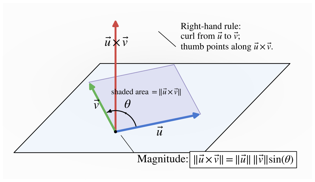
Illustration for the cross product \(\vec{u} \times \vec{v}\)

Example

Let \(\vec{u}=\langle 1,2,3 \rangle\) and \(\vec{v}=\langle 2,-1,1 \rangle\) in \(\mathbb R^3\).
Compute the cross product \(\vec{w}=\vec{u}\times\vec{v}\).
Verify that \(\vec{w}\) is orthogonal to both \(\vec{u}\) and \(\vec{v}\).

Solution

Compute the cross product \[ \vec{w} = \vec{u}\times\vec{v} = \langle 2\cdot 1-3(-1),\; 3\cdot 2-1\cdot 1,\; 1(-1)-2\cdot 2 \rangle = \langle 5,5,-5 \rangle. \]
Check orthogonality with \(\vec{u}\): \[ \vec{w}\cdot\vec{u} = 5\cdot1+5\cdot2+(-5)\cdot3 = 5+10-15 = 0. \]
Check orthogonality with \(\vec{v}\): \[ \vec{w}\cdot\vec{v} = 5\cdot2+5(-1)+(-5)\cdot1 = 10-5-5 = 0. \]
Therefore \(\vec{w}\) is orthogonal to both \(\vec{u}\) and \(\vec{v}\), as expected for the cross product.

Summary

Let \(\vec{u},\vec{v}\) be vectors in \(\mathbb R^3\). (Note: the cross products are only defined in 3D)
\(\vec{u}\times\vec{v}\) is the vector perpendicular to both \(\vec{u}\) and \(\vec{v}\), whose direction is determined by the right-hand rule and whose magnitude equals the area of the parallelogram spanned by \(\vec{u}\) and \(\vec{v}\).
It can be computed conveniently using a \(3\times3\) determinant.
To better understand why the determinant produces the correct vector, see 3Blue1Brown :: Cross products in the light of linear transformations.

Other Applications

See Larson, Section 3.4, for additional applications:
- Adjoint matrices and the formula for the inverse of a matrix.
- Computing the area of a triangle and the volume of a tetrahedron.
- Finding equations of lines and planes in \(\mathbb R^3\).