Applications of SVD
Lecture 32
Recap
$$ % Colors
% Coordinate vectors and matrices
% Common sets
% Abstract vector symbols
% Norms / absolute value
% Optional: dot product spacing (looks nicer in slides)
% Operators $$
Singular values
Let \(A\) be an \(n \times m\) matrix.
Let \(\lambda_1, \ldots, \lambda_m\) be the eigenvalues of \(A^T A\).
Since these eigenvalues are all nonnegative, we can take their square roots.
The singular values of \(A\) are defined by \[ \sigma_i = \sqrt{\lambda_i} \ge 0 \]
By convention, we order them in descending order: \[ \sigma_1 \ge \sigma_2 \ge \cdots \ge \sigma_r \ge \sigma_{r+1} = \cdots = \sigma_m = 0 \]
Important fact: the number of nonzero singular values equals the rank of \(A\), denoted \(r = \mathop{\mathrm{rank}}(A)\).
Singular value decomposition (SVD)
Let \(A\) be an \(n \times m\) matrix. Then \[ A = U \Sigma V^T \] where:
- \(U\) is an \(n \times n\) orthogonal matrix,
- \(V\) is an \(m \times m\) orthogonal matrix,
- \(\Sigma\) is an \(n \times m\) rectangular diagonal matrix whose diagonal entries are \[ \sigma_1 \ge \sigma_2 \ge \cdots \ge \sigma_r > 0, \] followed by zeros, where \(\sigma_i\) are the singular values of \(A\).
Properties of SVD
Always exists: every matrix (square or rectangular) has an SVD.
Singular values come from eigenvalues of \(A^T A\) (or \(A A^T\)), so they are always \(\ge 0\).
Connection to eigenvectors:
- Columns of \(V = [\vec{v}_1, \ldots, \vec{v}_m]\) are orthonormal eigenvectors of \(A^T A\): \[ A^T A \vec{v}_i = \sigma_i^2 \vec{v}_i \]
- Columns of \(U = [\vec{u}_1, \ldots, \vec{u}_n]\) are orthonormal eigenvectors of \(A A^T\): \[ A A^T \vec{u}_i = \sigma_i^2 \vec{u}_i \]
Relationship between \(U\) and \(V\):
- For each nonzero singular value \(\sigma_i\), \[ \vec{u}_i = \frac{A \vec{v}_i}{\sigma_i}, \qquad \vec{v}_i = \frac{A^T \vec{u}_i}{\sigma_i} \]
- So \(A\) maps right singular vectors to left singular vectors (up to scaling).
\(\Sigma\):
- tells how much each direction is stretched (by \(\sigma_i\)).
Step-by-step geometric picture:
- \(V^T\): rotate/reflect input (via eigenvectors of \(A^T A\))
- \(\Sigma\): stretch/shrink
- \(U\): rotate/reflect output (via eigenvectors of \(A A^T\))
Rank connection:
- number of nonzero singular values = rank of \(A\)
Key contrast with diagonalization:
- diagonalization may fail or not exist
- SVD always works
- \(U\) and \(V\) are generally different (unless special cases like symmetric matrices)
Applications
Revisiting least squares approximation
- Suppose we want to solve \(Ax=b\). If \(A\) is invertible, the solution is straightforward as \(x=A^{-1}b\)
- However, in many cases \(Ax=b\) has no solution at all (for example, when the system is overdetermined with more equations than unknowns), and we use least squares approximation to find a best possible solution \(x^*\) such that \(\|Ax^*-b\|^2\) is minimized
- We learned that we can solve the so-called normal equation \[A^TAx^* = A^Tb\] which always has at least one solution
- Can we just generalize the “inverse”, denoted as \(A^\dagger\) (called the pseudoinverse), such that the solution \(x^* = A^\dagger b\) just like the invertible case?
- The answer is yes, and the construction uses singular value decomposition (SVD)
A pseudoinverse from SVD
- Let \(A\) be an \(n \times m\) matrix. Consider the SVD \(A = U\Sigma V^T\) which always exists regardless of invertibility of \(A\)
- Recall that \(U\) is \(n\times n\) orthogonal, \(V\) is \(m\times m\) orthogonal, and \(\Sigma\) is \(n\times m\) diagonal (rectangular) with nonnegative singular values
- If \(A\) were invertible (square and full rank), then \[A^{-1} = (U\Sigma V^T)^{-1} = (V^T)^{-1} \Sigma^{-1} U^{-1} = V \Sigma^{-1} U^T\] since \(U,V\) are orthogonal
- The only possible issue happens for \(\Sigma\), e.g. if it is not square or contains zero entries (which cannot be inverted)
- While not strictly invertible, geometrically \(\Sigma\) stretches some directions by certain positive factors (the singular values), so we can “reverse” that stretching when the factor is nonzero
- Define the “pseudoinverse” of \(\Sigma\), denoted by \(\Sigma^\dagger\), as the \(m\times n\) rectangular diagonal matrix whose diagonal entries are the reciprocals of the nonzero singular values, and zeros elsewhere
- Replacing \(\Sigma^{-1}\) with \(\Sigma^\dagger\), we can define the pseudoinverse of any matrix \(A\)
Moore-Penrose pseudoinverse
Let \(A\) be an \(n \times m\) matrix with SVD \(A = U \Sigma V^T\). Then the Moore-Penrose pseudoinverse \[A^\dagger = V\Sigma^\dagger U^T\] where \(\Sigma^\dagger\) is an \(m \times n\) rectangular diagonal matrix whose diagonal entries are \[ 0 < \frac{1}{\sigma_1} \le \frac{1}{\sigma_2} \le \cdots \le \frac{1}{\sigma_r}, \] followed by zeros, where \(\sigma_i\) are the singular values of \(A\).
Normal equation and Moore-Penrose pseudoinverse
- Suppose \(Ax=b\) has no solution.
- It turns out that \(A^\dagger b\) is the least squares approximation, so \(A^\dagger\) is a reasonable generalization of the inverse
- Note the least squares approximation \(x^*\) is obtained from the normal equation \[A^TA x^* = A^Tb\] and thus we need to check that \(x^* = A^\dagger b\) satisfies the equation
- Using the SVD \(A=U\Sigma V^T\), we compute: \[ A^TA = (U\Sigma V^T)^T(U\Sigma V^T) = V\Sigma^T\Sigma V^T \]
- Then \[ A^TA(A^\dagger b) = V\Sigma^T\Sigma V^T (V\Sigma^\dagger U^T b) = V\Sigma^T (\Sigma \Sigma^\dagger) U^T b \]
- Since \(\Sigma \Sigma^\dagger\) acts like a projection onto the range, this simplifies to \[ = V\Sigma^T U^T b = A^T b \]
- Hence \(x^* = A^\dagger b\) satisfies the normal equation and is indeed the least squares solution
Example
- Consider an overdetermined system: \[ A = \begin{bmatrix} 1 & 1\\ 1 & 2\\ 1 & 3 \end{bmatrix}, \quad b = \begin{bmatrix} 1\\ 2\\ 2 \end{bmatrix} \]
- There is no exact solution to \(Ax=b\) because the three equations are inconsistent
- Compute the least squares solution using the normal equation: \[ A^TA = \begin{bmatrix} 3 & 6\\ 6 & 14 \end{bmatrix}, \quad A^Tb = \begin{bmatrix} 5\\ 11 \end{bmatrix} \]
- Now compute the pseudoinverse using the SVD of \(A\)
- The singular values are approximately \[ \sigma_1 \approx 4.079,\qquad \sigma_2 \approx 0.600 \] so \[ \Sigma \approx \begin{bmatrix} 4.079 & 0\\ 0 & 0.600\\ 0 & 0 \end{bmatrix} \]
- One SVD of \(A\) is \[ U \approx \begin{bmatrix} -0.323 & 0.854 & 0.408\\ -0.548 & 0.183 & -0.816\\ -0.772 & -0.487 & 0.408 \end{bmatrix}, \qquad V^T \approx \begin{bmatrix} -0.403 & -0.915\\ 0.915 & -0.403 \end{bmatrix} \] with \[ A = U\Sigma V^T \]
- Therefore \[ \Sigma^\dagger \approx \begin{bmatrix} 1/4.079 & 0 & 0\\ 0 & 1/0.600 & 0 \end{bmatrix} \approx \begin{bmatrix} 0.245 & 0 & 0\\ 0 & 1.665 & 0 \end{bmatrix} \]
- The pseudoinverse is \[ A^\dagger = V\Sigma^\dagger U^T \] so numerically \[ A^\dagger \approx \begin{bmatrix} 1.333 & 0.333 & -0.667\\ -0.500 & 0 & 0.500 \end{bmatrix} = \begin{bmatrix} \frac43 & \frac13 & -\frac23\\ -\frac12 & 0 & \frac12 \end{bmatrix} \]
- Now solve using the pseudoinverse: \[ x^* = A^\dagger b = \begin{bmatrix} \frac43 & \frac13 & -\frac23\\ -\frac12 & 0 & \frac12 \end{bmatrix} \begin{bmatrix} 1\\ 2\\ 2 \end{bmatrix} = \begin{bmatrix} \frac23\\ \frac12 \end{bmatrix} \]
- Equivalently, solving the normal equation gives \[ \begin{bmatrix} 3 & 6\\ 6 & 14 \end{bmatrix} x = \begin{bmatrix} 5\\ 11 \end{bmatrix} \Rightarrow x^* = \begin{bmatrix} \frac23\\ \frac12 \end{bmatrix} \]
- Thus the least squares solution is \[ x^* = \begin{bmatrix} \frac23\\ \frac12 \end{bmatrix} \] and this minimizes \(\|Ax-b\|^2\)
- Using SVD, we obtain the same solution via \(x^* = A^\dagger b\)
- Interpretation: we are finding the best-fit line \(y = x_1 + x_2 t = \frac23 + \frac12 t\) to approximate the data points
Dimension reduction
- One important interpretation of SVD is that larger singular values encode the main structure (or important core features) of the data, while smaller singular values often encode fine details or noise
- This is analogous to Fourier approximation: low-frequency components capture the overall shape (coarse features), while high-frequency components capture fine details or noise
- In particular, by dropping small singular values (and their corresponding singular vectors), we can reduce the dimension of the data while preserving its essential structure
- This idea leads to low-rank approximation: instead of using the full SVD \[ A = U\Sigma V^T, \] we approximate it by keeping only the top \(k\) singular values: \[ A \approx U_k \Sigma_k V_k^T \] where \(k\) is much smaller than the rank of \(A\)
- This is called the truncated SVD and provides the best rank-\(k\) approximation of \(A\) (in least squares sense)
- Practical interpretation:
- Data compression (store fewer numbers)
- Noise reduction (discard small singular values)
- Feature extraction (keep dominant patterns)
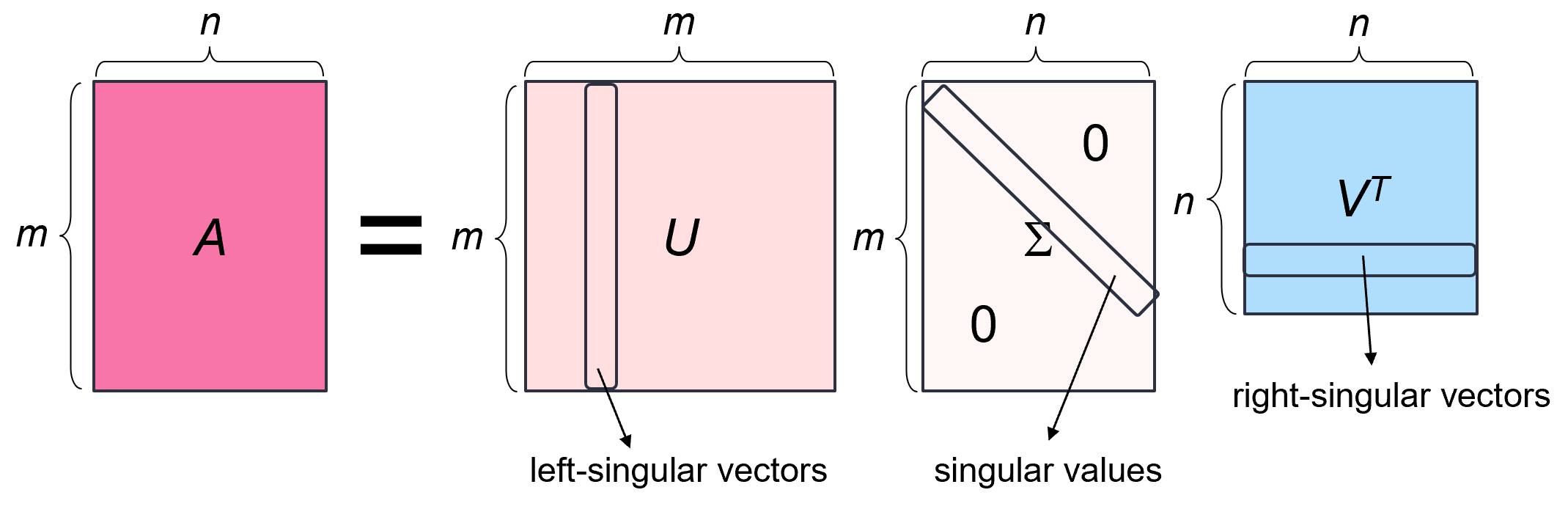
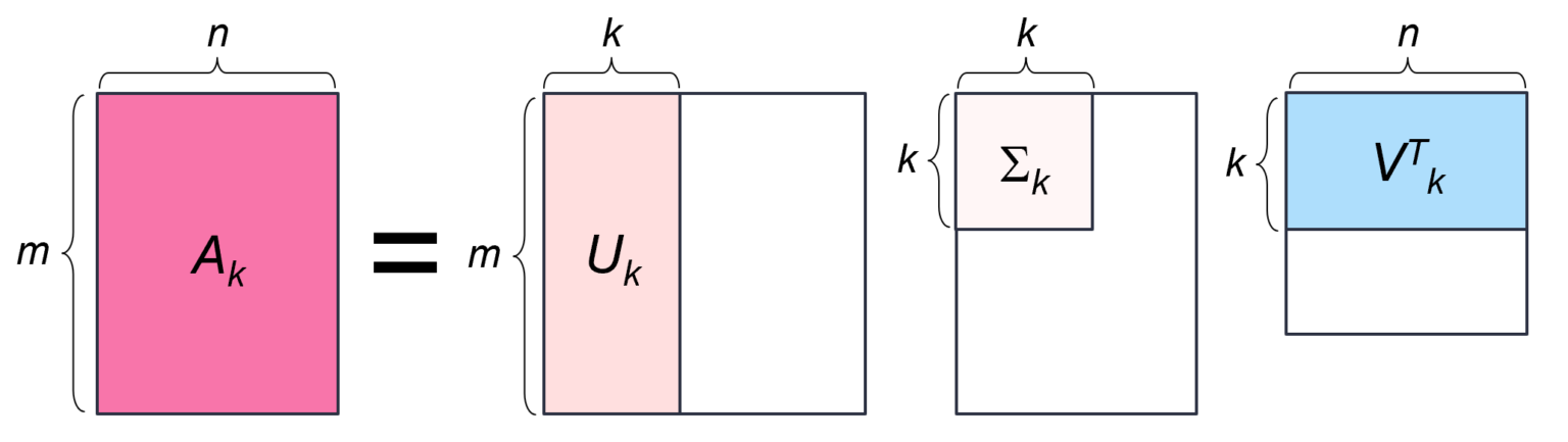 Image source: toward data science
Image recognition
- One of the most fun applications of SVD is image recognition
- While the demonstration in our class is elementary, modern industry applications (e.g., computer vision) build on the same core idea combined with machine learning
- The idea is as follows: for \(M\) images with \(K \times K\) pixels, we represent the dataset as a \(K^2 \times M\) matrix so that each column contains one image (flattened into a vector)
- We label them according to categories (e.g., digits, faces, objects)
- Given a new image (a \(K^2 \times 1\) vector), we want to find the closest data point to determine its category
- However, due to noise, lighting, and variation, directly comparing raw images is unreliable
- Here we use SVD to “compress” the data:
- Large singular values correspond to important features
- Small singular values often correspond to noise
- By keeping only the top singular values, we reduce dimensionality and improve robustness
- This process is also known as low-rank approximation or dimensionality reduction
Digit recognition
- Demonstration for digit recognition through SVD
- The exact same idea can be applied to face recognition or others
- A famous example is the Eigenface method, which uses principal components (from SVD) to represent faces efficiently
- See Wikipedia :: Eigenface