
Suppose I am collecting a sample of size \(n .\) Let \(X_1\) be the value of the first measurement, \(X_2\) be value of the second measurement, and so on. We assume that these variables are independent, normally distributed random variables with mean \(\mu\) and standard deviation \(\sigma.\) The sample mean is then normally distributed with mean \(\mu\) and standard deviation \(\sigma/\sqrt{n}.\)
Before the measurements are taken the sample mean is a random variable, and after the measurements are taken the sample mean is a fixed number. Sometimes this difference is indicated by denoting the sample mean before the measurements are taken with \(\overline X\) and afterwards with \(\bar{x}.\) For the sake of simplicity, I will denote both with \(\bar{x}.\)
You just bought a car. The dealer claimed that the car gets 250 miles on a full tank (10 Gallons). You suspect that the dealer was exaggerating and you decide to perform the hypothesis test \[\begin{align*} H_0 & : \mu \geq 250 \mbox{ vs.}\\ H_A & : \mu \lt 250 \end{align*} \] at significance level \(\alpha=0.05.\)
It seems that a natural choice for the test statistic would be the sample mean \(\bar{x}, \) where values of the sample mean much smaller than 250 discredit the null hypothesis. The problem is that the distribution of the sample mean depends on the parameter \(\sigma\) which is not known. The distribution of the standardized sample mean, \[T = \frac{\bar{x}-250}{s/\sqrt{n}},\] however, does not depend on any unknown parameter when \(\mu = 250.\) In fact, \(T\sim t(df=n-1)\) when \(\mu = 250.\)
The p-value is the probability of observing what has been observed or something more extreme in view of the alternative hypothesis. Values of \(\bar{x}\) that are much less than 250 correspond to values of the test statistic \(T\) that are much less than 0. Therefore the p-value is the area to the left of the observed value of \(T\) under the probability density function of the t-distribution with \(n-1\) degrees of freedom.
Suppose you measure the distance the car drives on a full tank and obtain the values 198, 222, 254, and 230. In this case \(T=-2.0785,\) and the p-value is 0.0646. Since the p-value is greater than 0.05 we fail to reject the null hypothesis. We have no evidence that the car drives fewer than 250 miles in average on a full tank. Does that confirm the claim made by the dealer? No, because the sample size might have been too small to detect the effect.
The p-value is always calculated under the assumption that the null hypothesis is correct. According to the null hypothesis \(\mu\leq 250.\) For the purpose of rejecting the null hypothesis the worst case
occurs when \(\mu = 250;\) this is why we use \(\mu = 250\) in our test statistic.
There are three different tests we can perform.
In each case the test statistic is given by
\[T = \frac{\bar{x}-\mu_0}{s/\sqrt{n}},\]
where \(\mu_0\) is called the hypothesized value of \(\mu, \) although it may just be the worst case
of the null hypothesis. In the example above \(\mu_0 = 250.\)
In the test \(H_0: \mu = \mu_0\) vs. \(H_A : \mu \neq \mu_0\) either large or small values of the test statistic discredit the null hypothesis. Suppose the observed value of \(T\) is \(t_0.\) Note that \(t_0\) may be positive or negative. The p-value in this case is the probability of observing a deviation from 0 as large as has been observed or even larger, that is, \[\mbox{p-value } = P(T\leq -|t_0|)+P(T\geq |t_0|), \] where the probabilities are calculated under the assumption that \(\mu=\mu_0.\)
Since the \(t\)-distribution is symmetric, it suffices to calculate the area in one of the two tails and double the result. In formulas, \[P(T\leq -|t_0|)+P(T\geq |t_0|)= 2P(T\leq -|t_0|) = 2P(T\geq |t_0|).\]
In the test \(H_0: \mu \leq \mu_0\) vs. \(H_A : \mu \gt \mu_0\) only large values of the test statistic, that is, values to the right of 0, discredit the null hypothesis. Suppose the observed value of \(T\) is \(t_0.\) The p-value in this case is, \[\mbox{p-value } = P(T\geq t_0). \] |
 |
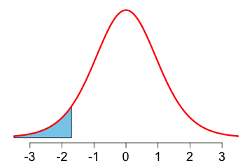 |
In the test \(H_0: \mu \geq \mu_0\) vs. \(H_A : \mu \lt \mu_0\) only small values of the test statistic, that is, values to the left of 0, discredit the null hypothesis. Suppose the observed value of \(T\) is \(t_0.\) The p-value in this case is, \[\mbox{p-value } = P(T\leq t_0). \] |
So far we have assumed that the data comes from a normal distribution. This assumption is not necessary for large sample sizes because of the Central Limit Theorem. As a rule of thumb we consider a sample size of at least 30 to be sufficiently large.
The formulas are easily evaluated using R. The number of measurements contained in a variable can be found with the function length(), the sample mean with the function mean(), the standard deviation with the function sd(), and a quantile of the t distribution with qt().
However, there is a better way than evaluating these formulas. Suppose you recorded the following mileages for your car: 198, 222, 254, and 230 miles. We assume that the mileage is normally distributed.
You can then calculate the p-value for the test \[H_0: \mu = 250 \mbox{ versus } H_A: \mu \neq 250\] using the following code.
| x = c(198, 222, 254, 230) | # store data |
| t.test(x, mu = 250) | # specify test |
Here is how you calculate the p-value for the test \[H_0: \mu \leq 250 \mbox{ versus } H_A: \mu \gt 250\]
| t.test(x, mu = 250, alternative = "greater") |
Suppose that you have a method for calculating a 95% confidence interval for the unknown parameter \(\mu.\) To be specific, suppose that \((198.8,253.2)\) is a 95% confidence interval for \(\mu.\)
Is there evidence that \(\mu\) is not 260? In other words, can we reject \(H_A: \mu = 260\) in the test \[H_0: \mu = 260 \mbox{ versus } H_A: \mu \neq 260\mbox{?}\]
Yes, because 260 is not in the confidence interval. One can be 95% confident that \(\mu\) is in the interval \((198.8,253.2)\) and since \(260\) is not in that interval, it is doubtful that \(\mu=260.\)
Is there evidence that \(\mu\) is not \(250\)?
No, because \(250\) is in the confidence interval. All we know from the confidence interval is that we can be 95% confident that \(\mu\) is between \(198.8\) and \(253.2.\) Since \(250\) is in that range, there is no evidence that \(\mu \neq 250.\)
Could we use the two-sided confidence interval to perform a one-sided test? More specifically, would the two-sided 95% confidence interval \((198.8,253.2)\) of \(\mu\) be evidence for \(H_A: \mu \gt 260\) in the test \[H_0: \mu \leq 260 \mbox{ versus } H_A: \mu \gt 260\mbox{?}\]
No, because the null hypothesis contains values that lie in the confidence interval. For example, the value 200 is contained in both, the null hypothesis and the confidence interval. However, the two-sided 95% confidence interval \((198.8,253.2)\) of \(\mu\) would be evidence for \(H_A: \mu \lt 260\) in the test \[H_0: \mu \geq 260 \mbox{ versus } H_A: \mu \lt 260,\] since the confidence interval does not contain any values of the null hypothesis.
We considered three types of hypothesis tests and three types of confidence intervals. It turns out that there is a correspondence between confidence intervals and hypothesis tests.
| confidence interval | hypothesis test |
|---|---|
| two-sided | \(H_0: \mu =\mu_0\) vs. \(H_A: \mu \neq\mu_0\) |
| lower-bound | \(H_0: \mu \leq \mu_0\) vs. \(H_A: \mu \gt \mu_0\) |
| upper-bound | \(H_0: \mu \geq \mu_0\) vs. \(H_A: \mu \lt\mu_0\) |
Using the decision rule based on the appropriate confidence interval is just as good as using the decision rule based on the p-value.
Recall the definition of the p-value.
This definition may appear to be clumsy but there seems to be no simpler way to say it. Suppose the p-value of a test turns out to be 0.0231. How do we interpret that value?
Unfortunately there is no single unified theory on statistical testing that all statisticians agree upon. Statistical testing is a mixture of ideas that have their roots in two different schools of thought that are at odds with each other. There are in fact, two approaches for interpreting the p-value.
Alternatively, we can interpret the p-value as a measure of evidence against the null hypothesis. Rather than drawing a conclusion based on a particular cutoff point such as \(\alpha=0.05,\) we report the p-value and comment on the strength of its evidence. In this approach, the smaller the p-value, the greater the evidence against the null hypothesis. The following suggestion on interpreting the size of a p-value is taken from Ramsey and Shafer, The Statistical Sleuth, p.47.
| p-value | 0 — 0.01 | 0.01 — 0.05 | 0.05 — 0.1 | 0.1 — 1.0 |
|---|---|---|---|---|
| evidence | convincing | moderate | suggestive | none |
Here is an example that illustrates the two approaches.
In 1868, the German physician Carl Reinhold August Wunderlich reported the mean body temperature to be 37.0 Celsius (98.6 Fahrenheit). Was Wunderlich wrong?
In this scenario the appropriate hypothesis test is \[ H_0: \mu = 37\quad \mbox{ vs. } \quad H_A: \mu \neq 37.\]
In order to perform this hypothesis test you need to collect measurements from a representative sample.
Download the data given in the link data.csv and read it into R using the function read.csv(). Be sure to set your Working Directory
to the location containing the data file.
| myData=read.csv('data.csv') |
| t.test(myData$temperature, mu=37) |
Approach 1. The mean human body temperature is significantly different from 37 Celsius (one-sample t-test; \(\alpha = 0.05\)).
Approach 2. There is overwhelming evidence that the mean human body temperature is not 37 Celsius (one-sample t-test; \(\mbox{p-value}\lt 0.0001\)).
In this example either result is rather useless. I don't think that anyone would have believed before the test was done that the body temperature is exactly 37 C or any other number for that matter. In this situation a confidence interval is much more useful since it gives us some information about the location of the body temperature.
If the null hypothesis is correct, one might think that small
p-values are less likely than large
p-values. It might come then as a surprise that the distribution of the p-value is uniform over the interval \([0, 1].\) In particular, it is just as likely for the p-value to be between 0 and 0.05 as it is to be between 0.05 and 0.1 when the null hypothesis is true. This is why in the first approach we have to specify the significance level \(\alpha\) before we look at the p-value and use that significance level as a cutoff point. For example it would not be appropriate to decide on \(\alpha=0.01\) and upon discovering that the p-value is 0.02 change the significance level to \(\alpha=0.05.\)
The second approach is more flexible. In this approach a p-value of 0.049 is not much different from a p-value of 0.051 since there is no cutoff point. The downside is that we cannot make any claims about the type I error rate.
Suppose only results that are significant at significance level \(\alpha=0.05\) are published. Can we say anything about the proportion of the published results that are actually true?
Unfortunately, we cannot. Here is an example to illustrate the point. Suppose 290 experiments are performed and in 200 of them the null hypothesis is true. Since the error rate is 5% when the null hypothesis is true, about 10 results are published that are wrong. If all the remaining 90 experiments correctly reject the null hypothesis, 100 results will be published and 10% of these are false. Since we don't know the proportion of false hypotheses being tested, we cannot know the proportion of correct published results.
You may be required to report your findings in APA format when writing a report or a paper for publication. Consider again the example of human body temperature. The result of the one-sample t-test could be reported as follows.
A one-sample t-test was conducted to determine whether the mean human body temperature differed from the hypothesized value of 37 °C. The results showed that the mean (M = 36.69, SD = 0.38) was significantly different from the hypothesized mean, t(99) = -8.25, p < .001, d = -0.83. The 95% confidence interval for the mean was [36.61, 36.76].
Note.