12.  Incorporating Phylogeny

MorphoJ can be used to map shape data onto phylogenies using squared-change parsimony (Maddison 1991). There is also a permutaiton test to determine if the morphometric data contains phylogenetic signal or not. Phylogeny files are imported into MorphoJ in the NEXUS file format. For this section we will be using Lythrurus.NTS data file.

Mapping onto phylogeny:

First you must have a phylogeny.  Ideally, this phylogeny should have branch lengths, as branch lengths provide a better estimate for ancestral values in squared-change parsimony.  This phylogeny can be created in most phylogenetic programs by saving the output tree with branch lengths.  You cannot simply build this tree, but must have the original dataset input into the phylogenetic programs and can then build the tree.  The taxa in the tree must match those in the shape analysis.  Tree files can be edited in text reading programs.

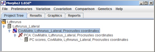
To map a phylogeny onto shape data, the first step is to import a phylogeny file as NEXUS tree format (.tre). Before that everyone needs to make sure the project has PCA done so the main user interface looks like the following:

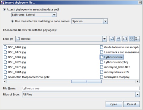
To import the phylogeny file click on File menu and click on Import Phylogeny File, which opens the following user interface:

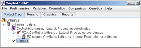
There are two buttons to choose the current dataset and choose the classifier. For this example the dataset is Lythrurus_Lateral and the clasifier is species have been selected. The choose the tree file and select Open. When the tree opens the project tree window looks like the following:

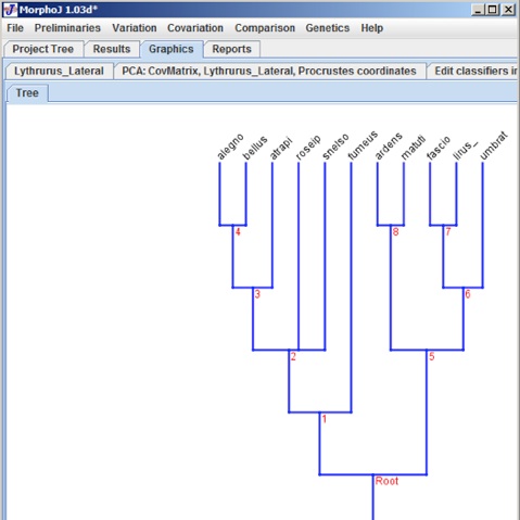
In this Project Tree the Phylogeny Tree is saved as Stored 1, to have an appropriate name for the tree, user can change it in the Nexus file. To check if the Phylogeny Tree has been imported proeprly a left mouse click on Stored1 and selecting Display Graphs shows the following dialog box:

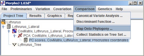
To map morphometric data onto phylogeny, select  PC scores in the project Tree window and select Map onto phylogeny under Comparison menu. The user interface would look like the following:

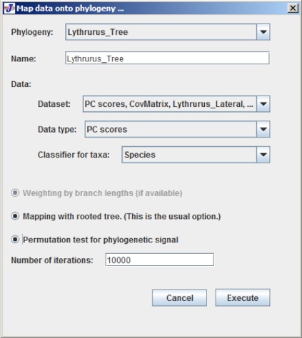
After selecting PC Scores, the following dialog box appears:

At the very top of the dialog box there are a few text boxes that give an option to choose the dataset and phylogeny tree.

The last button is Permutation test for phylogenetic signal which starts with the null hypothesis of not having any phylogenetic signal in the data set.

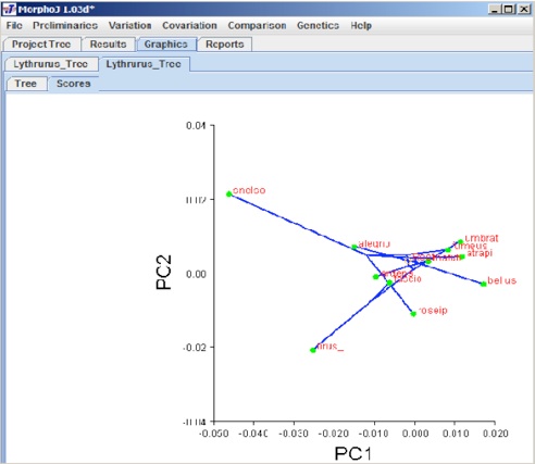
After all these selections click Execute and the following graphical user interface appears:

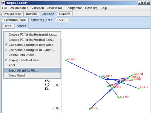
The graphical presentation depends on what kind of dataset has been used to overlay the phylogeny. A left click anywhere in this window gives a popup menu. This popup menu can be used to change the orientation of graph, scale factor, which PC axes to show, and to export the graph file and save it.

In this example we have mapped phylogeny tree on the PC data. Selecting the Result tab gives the result for this analysis and you can find the results of the permutation test. For this result the P-value = 0.7355, so no phylogenetic signal. Phylogeny can be mapped also onto Canonical Variates.

NEXT: Conclusion