Working paper · Pilot online edition · August 2026
The Effects of the National War Labor Board on Labor Income Inequality
The paper in brief
Can temporary wage controls reshape inequality decades later?
During World War II, the federal government limited raises using wage ceilings that varied across occupations and places. This paper links those historical “brackets” to Census earnings records and asks whether the policy left a durable mark on the wage distribution.
What we find
In 1979—more than thirty years after the policy ended—higher brackets were associated with slower growth in the earnings gap between the 50th and 90th percentiles. The evidence for the gap between the 10th and 50th percentiles is less clear.
Why unions matter
The lower-tail compressive effect is stronger where union density was higher. That pattern is consistent with unions carrying the wartime brackets forward as reference points in later wage bargaining.
How to read it
The estimates show persistent associations created by detailed variation in the bracket policy; they do not imply that every wartime wage control reduced inequality in the same way. The paper treats union bargaining as a plausible mechanism and identifies direct evidence on wage scales as a next step.
Abstract
During World War II, the United States federal government instituted an explicit policy of wage controls, which specified maximum allowable raises for those earning less than a certain level (the “bracket”) and froze wages for those earning more. We find that in 1979, three decades after the policy ended, higher brackets were associated with slower inequality growth as measured by the log ratio of the 50th to 90th percentiles of labor earnings. However, the effect on inequality at the bottom as measured by changes in the 10–50 log ratio was more ambiguous. The lower-tail compressive effect of the brackets was stronger where union density was higher, consistent with a role for unions in perpetuating the effects of the bracket through the wage bargaining process.
01
Introduction
The United States experienced a great compression in economic inequality between 1939 and 1969, with inequality falling sharply along many dimensions. Ever since, economists have been searching for the causes of this startling change in the income distribution. Goldin and Margo (1992) point to the wage controls imposed during WWII by the National War Labor Board (NWLB) as one possible explanation. While having antecedents in the policy responses to WWI and the Great Depression, the NWLB was an experiment of unprecedented scale and scope. At its height, the NWLB ostensibly controlled wages for the vast majority of workers in the private economy through what was known as the “bracket” policy. The policy allowed, but did not require, a wage below a specified level known as the bracket to rise to that level. At the same time, the policy forbade any raises, but did not require cuts, for those earning above the level of the bracket.
Our goal is to provide evidence on persistent effects of the NWLB on one dimension of inequality: the variation of wages within occupation by geography groups. To do this, we exploit variation across occupations and regions in the level of the bracket. In theory, brackets were supposed to be set as a function of the earnings distribution in the middle of 1943. For a given occupation, industry, and geographic location, the bracket was supposed to be equal to either the first “cluster” of wages or 90% of the mean wage, but these were never legally binding rules. In practice, the actual setting of the brackets resulted in substantial variation in the position of the bracket relative to the pre-war wage distribution.
Because our design relies on variation by occupation and county, we cannot use the publicly available Current Population Survey or even the IPUMS samples from the decennial censuses. Instead, we use the confidential full count decennial Censuses between 1960 and 2000 available through the Census Bureau’s Research Data Centers (RDC).2 Because of data limitations we discuss later, we focus on white-collar and metal trades occupations. We construct measures of inequality in labor earnings at the occupation-county level and regress changes from 1939 on the bracket and a host of controls including, among others, occupation and county fixed effects.
Theoretically, the marginal effect of an increase in the bracket depends on where the bracket is set in the earnings distribution. For example, consider the change in the log difference of the 10th and 90th percentiles of the earnings distribution, \(\Delta \log q_{10,90}\). If the bracket is set at the 10th percentile, the marginal effect of an increase in the bracket is positive, meaning that it slows the growth in inequality: the bracket locks in place earnings for the top 90% of the distribution while allowing the bottom 10% to receive a raise. If instead the bracket is initially set at the 90th percentile, the marginal effect is negative, since further increases in the bracket allow earnings at the top of the distribution to grow while leaving earnings at the bottom unaffected. Therefore, we estimate models separately for changes in inequality at the top and bottom and include the bracket and the bracket squared to capture the potential non-monotonic effect of the bracket.
We find that the brackets had persistent effects on inequality for decades after the end of the war and the NWLB, particularly at the top of the earnings distribution as measured by changes in the 50-90 gap. To understand the magnitude of the effects, we calculate the marginal effect of an increase in the bracket at different points in the distribution of brackets. As one example, the marginal effect in 1959 calculated at the median of the bracket was \(0.070\). To put that in perspective, a one standard deviation increase in the log bracket can explain 1/4 of the decrease in inequality at the top of the earnings distribution between 1939 and 1959. By 1989, the marginal effects are no longer statistically significant, suggesting that the effects of the brackets fade out over time. For inequality at the bottom of the earnings distribution as measured by the 10-50 gap, we find evidence of a non-monotonic effect of the bracket through 1979. Like for inequality at the top, any statistically significant marginal effects on inequality at the bottom disappear by 1989.
The results for inequality at the bottom cannot be explained by the simplest theory of how the brackets operated. For example, in 1969, the marginal effect on the change in the log 10-50 gap at the 10th percentile of the bracket distribution is strongly negative. This means an increase in the bracket from this level either reduced how fast the 10th percentile of wages grew or increased how the 50th percentile did. At the same time, the marginal effects at the 75th or 90th percentiles of the bracket distribution are strongly positive. We interpret these results as evidence that the brackets impacted not simply those earning just less than the bracket.
We also examine whether the brackets affected demographic dimensions of inequality. In principle, the brackets were supposed to apply uniformly to all races. If this policy was actually followed, then marginal increases in the bracket would reduce the within-occupation racial gap. What this means for the overall racial gap is not so easy to see because Blacks and whites did not tend to work the same jobs. How the brackets affect the between-occupation component of the racial gap is an empirical question that depends on the empirical relationship between the mean and dispersion of earnings. We find at most limited evidence of effects on the within-occupation racial gap. We also find some evidence that the brackets affected growth in the high school graduation earnings premium through 1979.
It is interesting to contrast the effects for the NWLB with those for another wage control policy during the war that capped salaries of the very top earners. The policy limited labor earnings to $25,000 after federal income taxes were paid. It also prohibited salaries of more than $5,000 from rising above their September 15, 1942 level. The first salary cap policy was repealed by Congress within 6 months after it was introduced. However, the prohibition on salary raises remained in effect until November 1946.3 Frydman and Molloy (2012) find that while in effect, this policy did reduce the growth rate of executive compensation. However, within a decade of the end of the policy, real average CEO compensation had recovered to its prewar level.
How then did the NWLB’s wage standards still impact earnings in the 1970s? We argue that unions played an important role in the persistence of effects.4 We provide both qualitative and quantitative evidence. To quantitatively test the role of unions, we extend our basic specification to include the interaction of the bracket with a measure of union density. We find the effect of the bracket on inequality in the bottom of the earnings distribution was greater for more unionized groups. This suggests that unions “locked in” the effect of the brackets after legal enforcement ended.
Our work fits into several distinct literatures. First, it contributes to the debate on the causes of the large swings in economic inequality during the 20th century. There are two broad categories of explanations for the changes. One set of explanations, as in Juhn et al. (1993), Katz and Murphy (1992), and Bound and Johnson (1992), focuses on the supply of and demand for different types of labor. For example, Autor et al. (2008) argue that a combination of a rise in skill-biased technical change and a deceleration in the growth rate of the relative supply of highly educated workers can explain the changes in the (educational) skill premium over the 20th century. Goldin and Katz (2009) argue that the “race” between education and technological change has been a defining feature of the American labor market for centuries.
An alternative set of explanations for these changes in inequality points to institutional changes, such as the minimum wage and unions. For example, DiNardo et al. (1996) provide evidence that changes at the bottom of the wage distribution during the 1970s and 1980s are consistent with an eroding real value of the minimum wage. Lee (1999) also argues that the minimum wage played an important role in “masking” increases in latent earnings inequality during this period.5 Finally, our work contributes to the literature on the consequences of WWII for economic inequality.6
The closest work to ours is the third chapter of the dissertation by Rose (2009). He too examines the effects of the NWLB on the wage distribution. However, there are important differences between that work and ours. First, we estimate effects many decades after the NWLB ended whereas Rose stops in the 1950s. Second, Rose only focuses on one particular region of the NWLB covering Arizona, California, and Nevada. In contrast, we cover most of the country. Third, we use a different identification strategy than Rose.
02
History of the NWLB and the Bracket Policy
The NWLB was established by an executive order on January 12, 1942. Its overarching goal was to aid the war effort, broadly defined.7 In particular, the NWLB hoped to promote “wage stabilization” (United States Department of Labor 1949, 178, volume 1), which, in concert with the controls on the prices of goods, was meant to help control inflation. In addition, the consequence of wage stabilization was “to help control the movement of manpower into war production” (United States Department of Labor 1949, 182, volume 1) as George W. Taylor, the chairman of the NWLB, put it in an April 1945 speech.
The goal was to prevent examples such as the following: “The production program in one area called for 2500 skilled employees of a certain trade […] Employers started bidding for them […] But there were still just 1500 skilled workers available. As a result of the bidding—they were made more mobile, more volatile, and less productive.”
The first labor dispute settled by the NWLB came within a month of its creation in the Aluminum Company case of February 1942, approving a wage increase of 7 cents per hour for Southern aluminum plants. On July 16, 1942, the NWLB resolved the “Little Steel” case, which was a consolidation of cases involving four steel companies, and established an explicit wage-stabilization formula. Based on a measured 15% increase in the cost of living between January 1, 1941 and May 1, 1942, the NWLB stated that “if any group of workers averaged less than a 15 per cent increase in hourly wage rates during or immediately preceding or following this period, their established peace-time standards have been broken. If any group of workers averaged a 15 per cent wage increase or more, their established peace-time standards have been preserved.” The result was the “Little Steel” formula that limited raises to workers who could show that they enjoyed a less than 15% raise over the preceding period. Implicit in the formula was that these workers could not end up receiving a raise of more than 15%, and workers who had received a raise of 15% or more before were not required to take a pay cut. This policy structure of not requiring pay cuts or raises but capping how much more people could earn would form the basis of the bracket policy.
At its inception, the jurisdiction of the NWLB was not clearly defined, and its charge to manage wages and settle disputes overlapped with other federal agencies such as the National Labor Relations Board and the Treasury’s Salary Stabilization Unit. Until the middle of 1942, the NWLB had only been involved in handling wage disputes between employees and employers. An executive order on October 3, 1942, drastically increased the jurisdiction of the NWLB to cover the vast majority of voluntary wage adjustments in private businesses. The only workers exempt from the NWLB’s jurisdiction were “those in establishments with eight or fewer employees (except certain classes removed from exemption from time to time), those employed by State and local Governments, and those employed by non-profit organizations.” The NWLB estimated in March 1944 that of 38 million total civilian non-agricultural employees excluding domestic servants, about 32 million were covered by executive order, and of these, 7 million were exempt by general order (United States Department of Labor 1949, 538). With this increase in the reach of the NWLB along with the implementation of the “Little Steel” formula, eight (and later twelve) regional offices were set up to adjudicate an anticipated flood of applications for wage adjustments. These offices initially had limited autonomy to settle disputes, but by early 1943, they gained a measure of freedom from Washington (Record 1944a). This freedom included “correct[ing] maladjustments within the 15% rule in specifically designated industries” and making decisions (subject to review) “if not more than 15% of the working force is involved, if no more than five cents is being given to any one employee and if the company does not use the increase to obtain relief from its price ceiling” (Hachenburg 1942, 354). These regional offices over the course of their lifetime would end up “process[ing] 463,000 applications for wage increases” (Goldin and Margo 1992).
Even with the Little Steel formula in place, a substantial rise in prices and wages forced President Franklin Delano Roosevelt to sign Executive Order 9328, also known as the “hold the line” order, in April 1943. The implementation of the “hold the line” order was through what came to be known as the bracket policy based on a subsequent May 12 directive. It authorized the NWLB to establish “by occupational groups and labor market areas, the wage-rate brackets embracing all those various rates found to be sound and tested going rates,” and, furthermore, “except in rare and unusual cases […], the minimum of the going rates within the brackets” would be the end point of any wage adjustments.8 Wages above the bracket “could not be changed on the basis of gross inter-plant inequities” and were frozen in place. For example, if the bracket for machinists in Danville, Virginia, was 85 cents per hour, an employer could receive approval to raise a machinist earning 70 cents up to 85 cents, but could not use inter-plant inequity to give a raise to a machinist already earning 95 cents.9 However, the worker earning 95 cents was not required to take a pay cut back to 85 cents; the policy instead froze that person’s wage in place.
The bracket policy remained in place until the end of the war in August 1945.10 The NWLB continued operations for a time under new executive orders that “freed from the necessity of governmental approval all voluntary wage adjustments which employers indicated would not require price increases or which did not involve increased costs to the government” (Witte 1952). The NWLB was formally ended on December 21, 1945, with a successor agency, the National Wage Stabilization Board, taking its place. In operation for fourteen months, the new agency’s approval was required for “wage increases which employers were not willing to say they would not use as a basis for price increases” (Witte 1952).
Within five years of the end of the NWLB, the US had entered the Korean War, and just as in WWII, the federal government set up an agency, the Korean War Wage Stabilization Board, to regulate wages. The agency used a similar rule to the NWLB’s “Little Steel” formula to determine wages: “The basic policy of the Wage Stabilization Board during the Korean War period was to permit wage increases up to a point not higher than 10 per cent. Above the level prevailing on 15 January 1950, which was the equivalent of the advance in the cost of living” (Muntz 1955). With the end of that war and Korean War Wage Stabilization Board, the wartime model of wage controls disappeared.
The Bracket Setting Process
Given the convoluted history of the NWLB, it should not be surprising that the process by which brackets were determined was also not straightforward. At a high level, the brackets were to be set as a function of the prevailing wage distribution for an occupation in a certain geography (and potentially industry). For occupations, the NWLB classified workers using the 1939 Dictionary of Occupational Titles developed by the Bureau of Labor Statistics (BLS). Occupations were sometimes further subdivided into grades. While the NWLB had broad authority over almost all wages in the private economy, the number of occupations explicitly assigned a bracket was relatively small. As United States Department of Labor (1949) stated, “wage rate brackets were established for [only] key occupations in an industry in a labor market area.” The rationale behind this was that since, in the NWLB’s view, the entire wage structure within a workplace was based on a set of “key” jobs, the NWLB only needed to control the wages for those occupations, which served as “peg points” for the entire distribution of wages (United States Department of Labor 1949, 231, volume 1). As the Region XII director put it, “[t]his limiting of brackets to key jobs was not only an economy of time, but it resulted in preserving intra-plant relationships more accurately than would have been the case if brackets had been set for practically all jobs” (United States Department of Labor 1949, 98, volume 3).
As for geography, the 12 NWLB regions were further divided into zones across which the bracket varied. In general, a zone was supposed to correspond to a “labor market area” (United States Department of Labor 1949):
[Such an] area encompassed by a particular bracket rate was normally a single locality but no hard and fast rules were applied with regard to geographical coverage. When determining the appropriate geographical area for a bracket determination, consideration was given to the labor market areas established by the Bureau of Labor Statistics and the War Manpower Commission. In general, the geographical coverage of a set of brackets represented an economic unit within which there was competition for labor. For certain industries, the wage structure was such that uniform rates were established for an area covering a number of contiguous localities or even an entire region.
Because of this lack of a hard and fast rule on how to define the boundaries of a zone, regions differed in how zones were defined. For example, in Region IV, county borders were used as boundaries, while in Region I, zones were sometimes defined at the level of a town. In other cases, the records do not specify precisely the boundaries of the zones. For example, in Region V, covering Kentucky, Ohio, and West Virginia, brackets were only assigned to broad areas such as “Louisville,” without reference to what area exactly made up Louisville. In some cases, the borders of zones were occupation specific.
Brackets were also, in principle, defined by industry, meaning two people in the same occupation in the same area might face a different bracket depending on the industries they worked in. Like for occupations, not all industries were explicitly assigned brackets. There is no documentary evidence that these unlisted industries were not subject to the NWLB; there is also no discussion as to why these industries were not listed in the brackets or which brackets were to apply.11 Because of this issue of unlisted industries, we focus on “occupations common to a number of industries, for example, clerical positions, [for which] cross-industry brackets rates were sometimes established. Thus, one rate was usually set for typists in all industries in one area” (United States Department of Labor 1949). This allows us to sidestep the issue of unlisted industries at the cost of looking at a more limited set of occupations.
To estimate the prevailing earnings distribution for the purpose of determining the brackets, the BLS conducted surveys of local employers. Based on this distribution, Record (1944b, 576) claimed that “[t]he bracket […wa]s usually set [at] 10 per cent below the weighted average, or at the first significant cluster of going rates.” To emphasize, this policy was not determined by statute or executive order, but simply how the NWLB interpreted its mandate. Under what circumstances which of these two options was to be used was left unclear, as well as what constituted a “significant cluster” of wages. Unfortunately, we have no records on which method was used to set the brackets in any given case nor information on the local wage distributions that the NWLB used to set the brackets. Adding to the complexity, the policy did not strictly forbid wage adjustments above the bracket, as “of course, increases justified on the basis of maladjustments, intra-plant inequities, substandards, or the ‘rare and unusual’ criteria could be permitted irrespective of brackets” (Record 1944b). Goldin and Margo suggest that to further its mission of helping to prosecute the war, “the NWLB [...] allowed certain wage increases in war-related industries.”
With all these caveats in mind, Figure 1 maps the brackets for stenographers highlighting the geographic variation.12 First, there was variation in the bracket between groups of states as a function of the NWLB region, denoted by the thick black lines, in which a state is located. For example, the difference in the brackets between Louisiana and Mississippi is (at least partly) explained because Mississippi was in Region IV and Louisiana in Region VIII. At a finer geographic level, there was also between-state variation within a NWLB region. For example, the value of the bracket in Nebraska differed from the value in Iowa even though both were located in Region VII. Finally, there was between-county, within-state variation, most prominently in Region IV that covered many southern states.
03
Data
NWLB Records
We collect primary source records on the brackets set by the NWLB at the occupation-industry-geography level. These records are located all across the country at the regional branches of the National Archives as well as in the centralized NWLB records in the National Archives at Kansas City.13 We supplement these records with the “Manual of Going Rates”, which published brackets up to March 15, 1944.14 Note that the archival records, or “bracket summaries”, are more comprehensive when available. In particular, for all brackets with a date of enactment listed, 49% went into effect after March 15, 1944, meaning we would not observe them if we relied solely on the manuals. The bracket summaries list only the value of the bracket at the end of the war with no information about whether brackets were modified before then. We assume that the brackets remained unchanged after March 15, 1944, for the regions where we use the manuals to collect the brackets (Region XII in the Pacific Northwest and Region VI centered in Chicago).
Census of Population
Our outcome and control variables come from the “long form” of the federal Population Censuses taken in 1940, 1960, 1970, 1980, 1990, and 2000. Everyone enumerated in these years was asked to provide basic demographic information including age, sex, race, and marital status. A random sample of individuals was then asked to fill out the long form with a richer set of economic and demographic questions. Our key dependent variable is total wage and salary income, which we will also refer to as labor earnings or income. The long form also asked about a person’s occupation, which is critical for linking these records to the brackets, and weeks worked, which is critical for defining our working sample. These employment-related variables all refer to the year before the Census was taken, e.g., 1939 for the 1940 Census of Population.
There are a few issues with these data to keep in mind. First, as
mentioned above, only a random fraction of the population received the
long form. This fraction varied from 1/4 in 1960 to approximately 1/6 in
2000. Second, the labor income variable was top coded to preserve
anonymity.15 These top-coded observations are
not a major problem because we are not focused on inequality at the very
top of the income distribution, and no more than a few percent of the
observations end up being top-coded. Third, while the original census
forms recorded occupations and industries as raw strings, we use the
recoded version of these variables into the occ1950 and
ind1950 classifications. The benefit of using the recoded
occupation is that this makes matching occupations to the NWLB records
easier. The cost is the relative coarseness of the 1950
classification.
Unfortunately, we are not able to utilize the 1950 Population Census. Recently, IPUMS released a 100% sample. However, it warned that “estimate[s of] the current total and wage income values exactly match the intent of the form roughly 70–75% of the time. The magnitude of the differences ranges widely. Wages are underestimated twice as frequently as they are overestimated […] Researchers should be cautious when using these variables and should screen for outliers.” In a related paper (Vickers and Ziebarth 2025), we show that these underestimates are a particular problem for higher-earning occupations. Moreover, we show that the standard deviation of wages (by occupation) in the 100% is underestimated relative to the (correct) income variable in the IPUMS 1% sample. The problem with trying to use the IPUMS 1% sample is not just the obvious problem of its size but also that geographic information is restricted. Since it was created before the 1950 Census was completely released to the public in 2022, to maintain confidentiality, county of residence is reported for only about 20% of the observations in the original 1% sample of 78K observations.16
Sample Construction
In our analysis, we focus on the same sample as Goldin and Margo (1992). First, we restrict attention to men, ages 18–65. Individuals in this group have traditionally been in the labor force so any effects of the brackets over time will not be due to changes in the composition of those employed. If we had included women, for example, this would create a potential concern that changes in the effects of the brackets over time could be due to changes in the composition of women in the workforce as the overall rate of women’s labor force participation increased. We further restrict attention to those who worked at least 40 weeks last year (the year the labor earnings variable refers to). Also following Goldin and Margo, we require that individuals “earn[], on average, more than one-half the minimum wage [in that year] on a full-time basis.” In the 1940 Census with a minimum wage of $0.30 / hour, this works out to requiring individuals to have average weekly earnings greater than $6.17
We end up restricting the sample further because the occupational
classification used by the NWLB does not line up exactly with the
classification in the Census. Because of this difference, we focus on
two particular groups of occupations that do line up well: white-collar
and clerical jobs as well as jobs in the metal trades industries. These
occupations, which total 28 OCC1950 codes, have a number of
useful features.18 First, the group of white-collar
occupations was a cross-industry classification, meaning we do not need
to worry about differences in the brackets by industry. This is not the
case for metal trades occupations. However, it seems likely that the
level of a bracket for the occupation in that industry was informative
about how that occupation would be handled in other industries, so we
have chosen to take these brackets as applying across industries in a
given region. Second, it was common for these occupations to be
explicitly mentioned in the bracket records. For the 10 white-collar
occupations, two (bookkeepers and clerical and kindred workers (n.e.c.))
have a bracket mentioned in the NWLB records for at least 1600 counties.
Other occupations such as draftsmen were recorded in relatively few
brackets.
Obviously, our final sample is not representative of the original Goldin and Margo sample. First, Figure 2 shows that because of our occupational restrictions, our sample is relatively less white, lower paid, and less educated. We do not find much difference in terms of marital status or whether living in the South. Second, because not all occupations were explicitly mentioned in the bracket records, Table 1 reports the percentage of individuals (and counties) by occupation that have a bracket assigned relative to the total number of individuals (and counties) in the 1940 Population Census. Overall, across the occupations we focus on, we cover about 16% of all counties and about 31% of all people. These percentages vary a fair amount across occupations. For sawyers, only a few percent are represented in our sample. In the most commonly assigned occupation (bookkeepers, with 1740 counties with a bracket assigned), 52% of the individuals in 1940 in that occupation have a bracket assigned.19
04
Empirical Strategy
Before discussing our empirical specification, it is important to understand how the bracket policy functioned. The policy differed in an important way from a conventional minimum wage in that the bracket policy did not require firms to do anything. Firms did not have to give a raise to workers earning below the bracket nor cut the wages of workers earning more than the bracket. In this sense, the bracket operated as a “soft maximum” rather than a hard cap that made earning more than a certain level illegal. As a consequence, unlike an increase in the minimum wage, a higher bracket need not mechanically reduce inequality. Its effect depends both on where the bracket lies relative to the wage distribution and on the underlying trends in the wage structure.
Consider a scenario where wages are generally rising, a reasonable assumption for WWII and the postwar period.20 Split workers into three groups. In the first group are workers whose wage was already above the bracket. For them, a marginally higher bracket would not matter since their wages were already above the allowable adjustment. In the second group are workers whose wage absent the bracket altogether would still remain below the actual value of the bracket. Again for this group, a marginal increase in the bracket would have no effect. It is only for the third group of workers who earn an intermediate amount that a higher bracket has an effect. This group earns less than the bracket but close enough that, absent the bracket, they would have ended up earning more than it.
The consequence of this partition is that the marginal effect of the bracket will depend on where the bracket is initially set. Suppose, for example, that the bracket is set in the middle of the earnings distribution. Then marginally increasing the bracket allows wages in the middle of the distribution to rise over time while leaving wages both near the top and the bottom unchanged. Therefore, upper tail inequality, as measured by say the 50-90 gap, for example, would fall while lower tail inequality, as measured by the 10-50 gap, would increase. The overall effect on the 10-90 gap would then be muted because of offsetting effects on upper and lower tail inequality. On the other hand, if the bracket lies near the top of the distribution, then a marginal increase in the bracket would allow wages near the top to rise while leaving wages lower in the distribution unchanged. In this case, the effect of a marginal increase in the bracket is to increase overall inequality. Conversely, if the bracket was set near the bottom of the wage distribution, then a marginal increase in the bracket would have the opposite effect and reduce overall inequality.
This very simple, basically mechanical model of how the brackets operated is useful for interpreting our empirical results even though it abstracts from many potential complications. One potential complication is that changes in the bracket may have had spillover effects on those not directly affected by the bracket. This could be due to violations of the bracket policy with people earning above the bracket receiving raises. It could also be because those earning much less than the bracket receive an additional raise when the bracket is increased. This is akin to the hypothesized “ripple effect” often discussed in the context of the effects of minimum wages on inequality whereby those earning just above the minimum wage also receive a raise when the minimum wage is increased.21 Implicitly, the NWLB believed in such spillovers because it only set brackets for certain key occupations confident that controlling wages for those occupations would determine the whole wage distribution.
Denote the bracket for occupation \(i\) in county \(c\) by \(\bar w_{ic}\). Our outcome variable is the change between year \(t\) and 1939 in the log ratio of the \(\tau'\) and \(\tau\) percentiles of labor earnings for occupation \(i\) in county \(c\), denoted by \(\Delta_{ic} \log q_{\tau,\tau'}\). This is based on labor earnings, not the wage rate, even though the wage rate is what was actually controlled by the NWLB.22 For simplicity, we suppress the dependence of this variable on time. In all our specifications, we put the lower percentile in the numerator (\(\tau < \tau'\)), meaning the log ratio will be negative and a positive effect of the bracket reduces the growth rate of inequality. We estimate decade-by-decade the following specification: \[\begin{equation} \Delta_{ic} \log q_{\tau,\tau'} = \beta \log \bar w_{ic} + \gamma [\log \bar w_{ic}]^{2} + \text{Controls}_{ic} + e_{ic}. \label{eq:unconditional} \end{equation}\] We include both the bracket and its square to capture potential non-monotonic effects that depend on the level of the bracket. The controls are (1) county fixed effects, (2) occupation fixed effects, (3) the value of \(\log q_{\tau,\tau'}\) in 1939 and its square, and (4) the mean income by occupation-county in 1939.23 Because an “observation” is a statistic derived from a group of individuals in a given occupation-county cell, following Autor et al. (2016), we weight the observations by the total number of workers in that cell.24
Quantitative Evidence on the Bracket Setting Process
The causal interpretation of our regression relies on the claim that the residual variation in the bracket, after controlling for the underlying wage distribution, was as good as random. We support this claim by first showing that the local earnings distribution was strongly predictive of the bracket so that we can control for the systematic part of the brackets. Second and more importantly, we show that the residual variation in the brackets after controlling for the earnings distribution is not correlated with other local economic characteristics such as war spending that might be correlated with subsequent changes in inequality.
To start, we regress the brackets on various statistics at the county-by-occupation level of the 1939 hourly earnings distribution adjusted for growth in earnings of production workers between 1939 and 1943 (Officer and Williamson 2022). Ideally, we would use the contemporaneous distribution of earnings used by the NWLB in setting the brackets, but we do not have access to that information.25 To limit the influence of outliers, we winsorize the 5% tails of the hourly earnings distribution. The first column in Table 2 reports the \(R^2\) from a regression of the brackets on occupation and county fixed effects highlighting that nearly all the variation is explained by these two factors. Columns 2 through 4, which do not include occupation and county fixed effects, show that there are statistically and economically significant positive relationships between the bracket and the 10th, 25th, and 50th percentiles. This is consistent with the claim based on narrative evidence that the brackets were determined by the local wage distribution (albeit in a less than straightforward way). In Column 6, after including all of these statistics, we can explain about 16.5% of the variation in the brackets. The fact that this percentage is relatively low is, at least, partially due to the fact that we do not have the same information as the NWLB used to set the brackets.
Our biggest worry is that the residual variation in the bracket is correlated with other factors that might themselves be correlated with future changes in inequality. To study this possibility, we first examine in column 7 whether demographic characteristics including fraction married, age, fraction white, and fraction with a high school degree predict the bracket. Only the fraction white is statistically significant with the bracket. This is potentially evidence of racial bias in the bracket setting process. The last column of Table 2 includes proxies for the local war effort including military spending on production contracts as well as investment in facilities (Aizer et al. 2020) as well as state-level mobilization rates (Acemoglu et al. 2004). We also include state-level unionization rates (Farber et al. 2021) as another potential non-earnings related determinant of the brackets. We note that all of these additional variables only vary by geography and not by occupation (or industry).
We find some evidence that measures of military mobilization and the local war effort are correlated with the bracket, even after controlling for the wage distribution and demographic characteristics. The positive association between the bracket and combat supply contracts is consistent with the NWLB ensuring that areas heavily involved in the war effort would be able to set higher wages to attract workers though the actual economic significance of this association is very small. The state-level induction rate is also positively correlated with the bracket potentially, reflecting the need for higher wages in areas of relatively low labor supply because of high mobilization. On the other hand, the association with spending on industrial facilities as well as the unionization rate are economically insignificant. Including these war-related variables barely affects the \(R^2\), and the ratio of the residual variation relative to the variation in the bracket is just under 90%. In the end, we conclude that the local war effort had only limited effects on the bracket setting process after controlling for the local earnings distribution.
While not critical for identification, exactly where in the distribution of earnings the brackets tended to be set has important implications for the predicted marginal effects of the bracket.26 This is not a straightforward question to answer because as mentioned, we do not observe the distribution of earnings at the time the NWLB was setting the brackets. Given this limitation, we consider two hypothetical scenarios. In the first, we assume that the brackets were always set according to the 90% of the mean rule and calculate the distribution of the imputed brackets expressed as percentiles of the 1939 hourly earnings distribution at the zone by occupation level. Figure 3 shows that in this hypothetical, brackets tended to be set between the 20th and 60th percentiles. The fact that in some cases, even 90% of the mean is greater than the median or even the 75th percentile should not be surprising given the skewness of the earnings distribution. As a point of comparison, Rose reports that for a sample of occupations from Region X, that the brackets were usually in the bottom 20% of the hourly earnings distribution at the time.
The obvious problem with this hypothetical distribution of the bracket is that we have no evidence that the 90% rule was followed religiously. The NWLB reported that for Region III centered in Philadelphia, administrators tended to use the first cluster method, though “not exclusively” (United States Department of Labor 1949, 1176, volume 2). The analysis found “wide difference in individual occupations between the bracket rates set by the 10 percent [below the mean] method and the actual rates set”, but these differences “largely balance themselves” (United States Department of Labor 1949, 1177, volume 2) meaning brackets were not systematically higher or lower under one or the other method. Rose quotes one memo from NWLB Region X that stated: “In an analysis of 160 brackets set, the California regional board found 97 had been set by the cluster method and 17 by the ten percent method; in 4 cases, the cluster method and the 10% method generated identical results. This leaves 50 of 160 brackets which were set with some other criteria in mind.”
Our second hypothetical is to take the distribution of brackets however determined as given and impute the distribution of earnings when the NWLB was determining the brackets. We make this imputation by again adjusting hourly earnings in 1939 for production worker earnings growth between 1939 and 1943.27 Figure 4 plots for white collar and metal trades occupations the distribution of the percentile of the brackets in the imputed hourly earnings distribution. For white-collar workers, a substantial fraction of brackets fell in the bottom fifth of the distribution, and most were below roughly the 40th percentile. For metal trades workers, the picture is different. Nearly all the brackets were higher than the 20th percentile of the earnings distribution. One potential explanation for the difference between the two groups of occupations is that we are assuming too high of a growth rate in earnings between 1939 and 1943 for white collar occupations when using the growth rate of earnings for production workers.
05
Results
Effects on Changes in the 10-50 and 50-90 Gaps
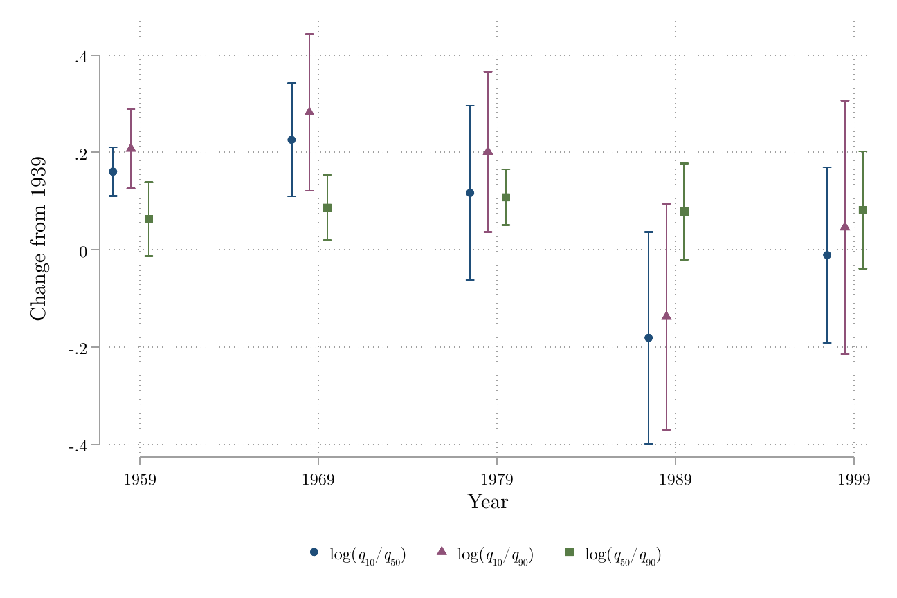
Figure 5 plots the linear and quadratic terms of the bracket for each of the Census years and the various percentile gaps. We find that the bulk of the coefficients for the different inequality measures are both positive and statistically significant through 1979, decades after the end of the NWLB.28 However, for the 50-90 gap, the quadratic term is small and usually insignificant, while the linear term is positive. Any statistically significant coefficients disappear by 1989.
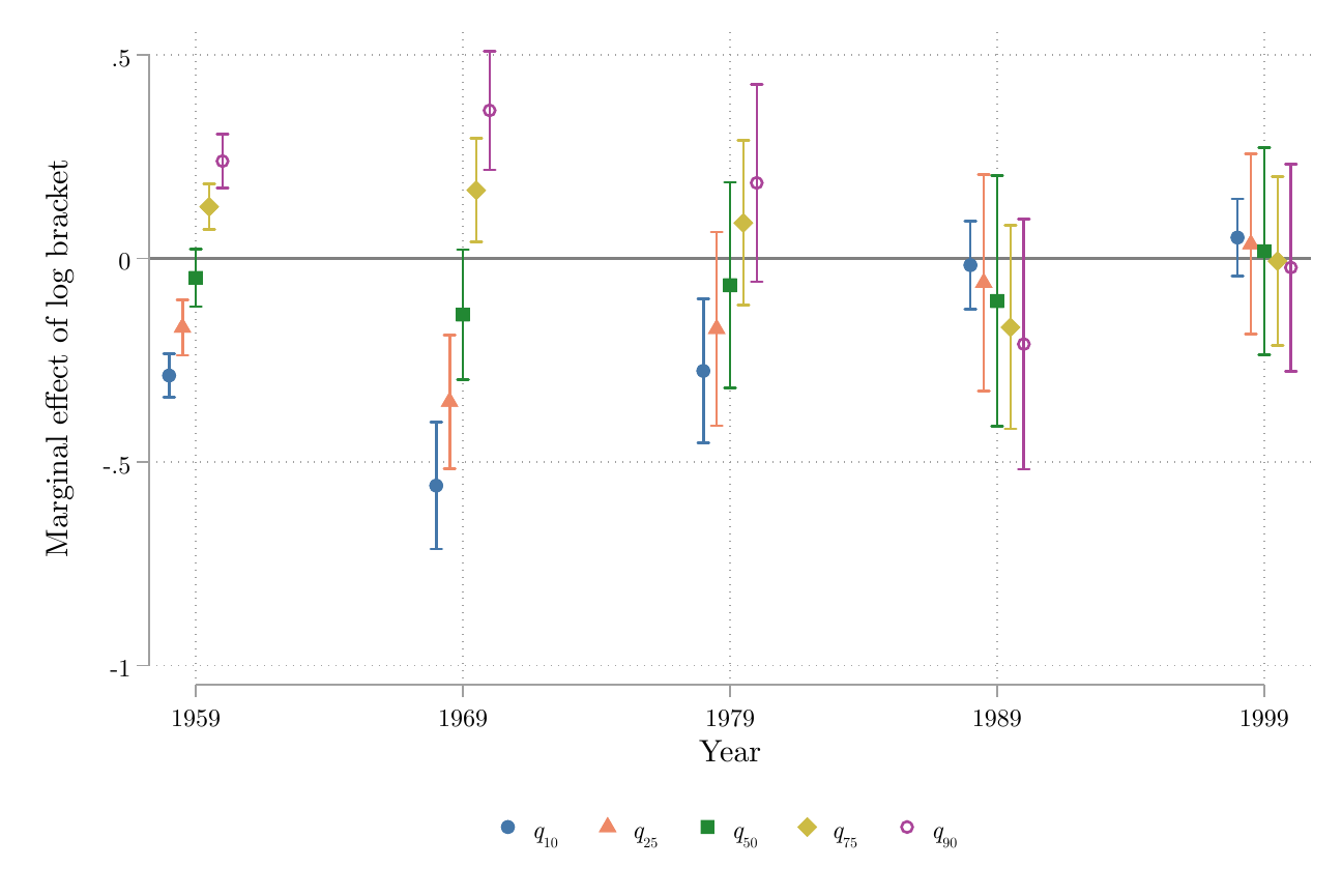
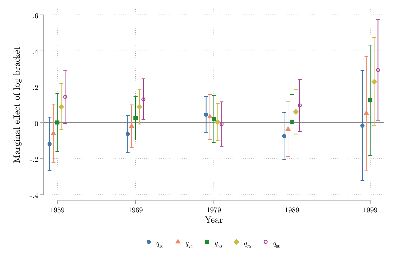
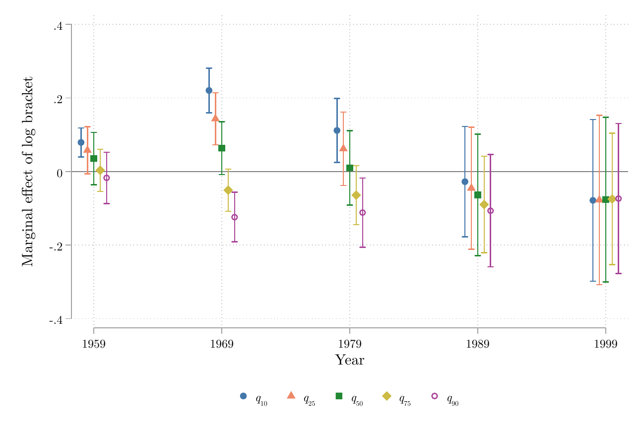
To interpret the magnitude of our results, we compute marginal effects with respect to the log bracket, the treatment variable in Equation (1). Because our regression specification is nonlinear, the marginal effect of an increase in the bracket depends on the level of \(\log{\bar{w}}\). In particular, the marginal effect is equal to \(\widehat{\beta} + 2\widehat{\gamma} \log \bar{w}\). We calculate the marginal effect of an increase in the bracket for the 10th, 25th, 50th, 75th, and 90th percentiles of the log bracket’s distribution.29 Thus, the reported marginal effects are with respect to a proportional change in the bracket, rather than a one-dollar increase in the bracket. Figure 6a shows that the marginal effects for the 10-50 gap in 1959, 1969, and 1979 differ in sign depending on the value of the bracket at which the marginal effect is evaluated. For values of the bracket low relative to the 1939 distribution of wages, the marginal effect of an increase in the bracket is to increase the growth rate in inequality at the bottom. This can be rationalized by an increase in the bracket allowing people in the bulk of the distribution to rise, while those very low in the distribution are unaffected since their wages were not subject to the bracket in the first place. Hence, inequality increases. In contrast, when brackets are set high in the distribution, the marginal effect of an increase in the bracket is to reduce inequality. On the other hand, the marginal effects for the 50-90 gap in Figure 6b are unambiguously positive. No matter the percentile of the distribution of brackets, the marginal effect is positive, meaning that a marginal increase in the bracket slowed growth in inequality at the top. Like the marginal effects for the 10-50 gap, the marginal effects here fade out (at least statistically speaking) by 1989. Nevertheless, it is striking that more than three decades after the end of the war and the NWLB, there are still detectable effects of the wage controls on inequality at the top and the bottom of the wage distribution.
As an example, consider the change in inequality of the 50-90 gap from 1939 to 1959. The standard deviation of the log bracket (weighted by the number of workers in 1940) was \(0.212\),30 and the marginal effect evaluated at the median was \(0.070\). Hence, a one standard deviation increase in the bracket leads to a \(0.015\) decline in the growth rate of inequality relative to the mean change of \(0.060\) over these two decades. Hence, a one standard deviation increase in the bracket explains about 1/4 of the decline in inequality at the top between 1939 and 1959. Note that, at least for this year and measure of inequality, the marginal effects were relatively similar no matter where the bracket was placed in the initial distribution (though as a percentage of the mean change, the magnitude of the marginal effect could be quite different).
Besides the persistence of the effects, there are some other surprising results from the viewpoint of the simple framework we laid out. First, in some years and at some values of the bracket, the marginal effects on inequality at the top and bottom are of the same sign. Second, it is surprising that for the 10-50 gap through 1979, the marginal effects are increasing in the bracket. Both of these sets of results are inconsistent with the assumption that changing the bracket only affects the wages of those earning just less than the bracket.
A related debate has arisen in the minimum wage literature about whether workers earning (somewhat) more than the minimum wage also tend to enjoy a pay raise from an increase in the minimum wage. The theoretical idea is that wages are (at least partially) determined through workplace hierarchies so that raises for people at the bottom require raises for those further up the earnings distribution to maintain the hierarchy. This view is actually quite similar to that of many people who ran the NWLB. The issue with applying this theory to our case is that unlike people who initially earned more than the minimum wage, people earning more than the bracket were (in principle) legally prevented from getting a raise.
Effects on Changes in Demographic Inequality
We now examine effects of the brackets on two demographic dimensions of inequality: the racial earnings gap and the educational skill premium.31 To be sure, we will be examining between group inequality within occupations and regions. The overall earnings gap between two groups depends not just on the gap within occupations (and regions) but also the gap in average earnings between the occupations (and regions) the groups tend to be in as well as sorting across the occupations. Clearly, for the racial and educational earnings gap, the between occupation piece is critical. Nevertheless, it is interesting to examine the within component of inequality since the NWLB explicitly stated that the brackets were supposed to apply uniformly regardless of race, age, gender, or educational attainment.32 In theory then, the brackets, assuming they were enforced uniformly, should have reduced inequality between demographic groups within occupation and county.
Based on the same specification as before, Figure 7a shows the marginal effect of the bracket on (minus) the racial earnings gap. Hence, a positive marginal effect means that an increase in the bracket reduces the change in log ratio of average earnings for whites to Blacks (within an occupation-county group). On the whole, we find limited evidence that the brackets reduced the (within) racial wage gap. These null effects could be because the brackets were not actually enforced uniformly or the racial gap within occupation and county was not important.33 If we take the differences in marginal effects for 1959, say, as meaningful, we again face the puzzle as for the 10-50 results that it was when the bracket was set higher that further increases reduced inequality. This is surprising since even within occupations, white workers earned more on average than Black workers, so an increase in the bracket should be relatively more beneficial for whites, who were higher earning to begin with.
Figure 7b examines the marginal effects on changes in the gap between the average wage of high school graduates compared to non-graduates. Again a positive marginal effect means that an increase reduces the growth in inequality between these two groups (within occupations and counties). Here we do find through 1979 results consistent with the fact that even within an occupation, the highly educated will tend to get paid more so the effect of a marginal increase in the bracket will tend to be enjoyed most by this group. Therefore, the marginal effects should be decreasing in the level of the bracket, which is what we find, and when the bracket is high enough, marginal increases serve to increase the growth in educational inequality, which is also what we find.
The Connection Between the NWLB and Great Compression
Addressing the connection between the NWLB and the Great Compression is a complicated question because the Great Compression was a multifaceted phenomenon. Not only did overall inequality fall, but inequality between education and occupation groups also fell and residual inequality conditional on observables like education also fell.34 In addition, a fraction of the decline in inequality was also due to shifts in the observable characteristics of workers (Goldin and Margo 1991). Our empirical strategy is not designed to address how the NWLB affected all these different dimensions. We are also only examining a limited set of occupations, and it is not clear whether our results would generalize to the whole population. Moreover, our data do not cover what happened during the war or the first decade after. Finally, there were other components of the NWLB such as a minimum wage that allowed blanket raises on the basis of “substandards of living.” Presumably, this would have decreased lower tail inequality at least during the war, but our design utilizing cross-region and occupation differences in the brackets will not capture such compression.
The dimension of inequality we can partially address is the residual or within component, which was an important part of the Great Compression. Goldin and Margo estimate that the 90-10 gap in residual wage inequality fell by about 16 log points between 1940 and 1960. This measure of residual inequality is slightly different from what we calculate since Goldin and Margo condition on many more observable characteristics such as education and experience.35 As for the “location” of the decline in residual inequality, Goldin and Margo find that about 1/3 is due to a decline in inequality at the top and the remaining 2/3 due to a decline in inequality at the bottom. Furthermore, they argue it was inequality at the top that declined during the war and postwar period while it was inequality at the bottom that declined between 1940 and the start of the war.
While pointing to the NWLB as one driver of the Great Compression, Goldin and Margo admit that it is hard to explain the decline in inequality at the top through “a simple application of the rules of thumb used by the NWLB, which allowed wage increases at the lower end of the distribution.” At least empirically speaking, our results resolve this tension since we find consistently compressive effects of the brackets on inequality at the top of the distribution. At the same time, we agree with Goldin and Margo that this decline did not come through a “simple application” of the brackets. While it is not easy to say where the brackets were exactly, all the evidence we have provided here as well as narrative evidence on the bracket setting process suggests that the brackets were set lower in the distribution so that marginal increases should not have affected inequality at the top of the distribution.
In the end, we do believe our results support Goldin and Margo’s claim that “the NWLB had large effects on the wage structure [even at t]he upper tail of the distribution” and the compression lasted long after the war was over. But what would the distribution of wages have looked like if there had been no NWLB? This is difficult to say since our design is not well-suited to addressing that counterfactual.36 Is such a counterfactual equivalent to setting the bracket arbitrarily high in our estimated regression model? Perhaps, but such a value is well outside the support of the actual distribution of the brackets. What is clear is that the NWLB’s brackets left fingerprints on the wage distribution long after the agency itself had disappeared. But how?
06
The Role of Unions
The leaders of the NWLB would not have been surprised to hear that the brackets had effects on the earnings distribution for decades after the war. While the fighting was still ongoing, George Taylor, the vice chairman of the agency, noted that the NWLB was “helping to develop collective bargaining by providing a vast reservoir of information about clearly defined job classifications and wage rate schedules from which the parties can draw facts relevant to their negotiations, both now and after the war” (National War Labor Board 1944, III).37 In line with Taylor’s thinking, we argue that an important channel through which the brackets affected wages for decades was the way in which the preexisting wage distribution acts as a reference point in wage negotiations.38 In this way, the direct effects of the brackets on the earnings distribution while they were legally binding during the war could have been locked in through the postwar wage bargaining process, particularly in cases of collective bargaining between businesses and unions.
Based on surveys of sixty unions, Levitan (1951) writes that “Three years after the War Labor Board ceased to exist, a number of unions found that it had left definite imprints upon the postwar job evaluation and individual wage rate structures in their respective industries. This seems particularly true of the steel industry. The War Labor Board served as a catalyst in stimulating the formulation of a much-needed job classification and rational wage rate structure in the steel industry.” A 1951 report of the Industrial Union of Marine and Shipbuilding Workers of America (Industrial Union of Marine and Shipbuilding Workers of America, CIO, Research Department 1951) explained one reason for persistence (emphasis added):
In 1943, 1944, and 1945 the Shipbuilding Commission of the National War Labor Board conducted extensive surveys of basic rates throughout the industry and evolved definite rate and wage structures for the trades in each shipbuilding zone. It is interesting to note that these structures have never been changed, even since the war—that the increases since the war have always been on an across the board level, because once the basic structure of the trades is tampered with in any shipyard, the entire delicate mechanism by which the trades are graded in accordance with the skills required, goes by the board.
We should also keep in mind that wage stabilization was brought back during the Korean War. We do not have direct evidence on effects of the Korean War version of the NWLB. Keat (1960) finds a still compressed between-occupation earnings distribution in 1956, three years after the dissolution of the Korean War Wage Stabilization Board.
Besides the leaders of the NWLB, many others have suggested that the brackets affected private wage setting through their effects on what is perceived as a fair wage.39 Thurow (1975) argues that “[existing wage] differentials became the new standard of relative deprivation and were regarded as ‘just’ even after the egalitarian pressures of WWII had disappeared.” Piketty and Saez (2003) also mention a similar mechanism when they write that “World War II without doubt had a profound effect […] on social norms regarding inequality.” Similar claims about the role of norms were made by Frydman and Molloy (2012), Goldin and Margo (1992), and much earlier by Brown (1977). No one likes to take a nominal pay cut.
For more direct quantitative evidence on the role of unions, we augment Equation (1) with the interaction between the bracket and a measure of unionization: \[\begin{equation} \begin{split} \Delta_{ic} \log q_{\tau,\tau'} &= \beta \log \bar w_{ic} + \gamma[\log \bar w_{ic}]^{2} + \theta_{1} \mbox{UNION}_{ic} + \theta_{2} \mbox{UNION}_{ic} \log \bar w_{ic} \\ & + \theta_{3} \mbox{WC}_{ic} \log \bar w_{ic} + \text{Controls}_{ic} + e_{ic}. \label{eq:unconditional_extended} \end{split} \end{equation}\] where \(\mbox{UNION}_{ic}\) is the measure of unionization and \(\mbox{WC}_{ic}\) is an indicator for whether the occupation is white-collar.40 The problem we face is that the Census does not report union status, so we calculate the unionization rate by state and occupation using data from Farber et al. (2021) and, when available, the Current Population Survey.41 The unionization rate varies by time so there is a potential endogeneity concern if the bracket itself encouraged (or discouraged) unionization. The unionization measure is also imprecise since it only varies by state and 1-digit occupational groups. Unfortunately, this is the best we can do with the available data.
We report the union interaction term in Figure 8 for various measures of inequality and years. While somewhat noisy, there is a clear pattern that the effect of the interaction between unionization and the bracket is positive for the 10-50 ratio.42 This means that the bracket had a stronger effect on compressing the lower part of the earnings distribution in occupations and counties where unionization was higher.43 To be clear, this does not mean that unionization alone led to compression in the lower part of the earnings distribution, rather unions interacted with brackets to reduce inequality for decades. To gauge the magnitude of the interaction, consider a one-standard-deviation increase in the log bracket. At the mean unionization rate in 1979, the interaction term implies an additional 1.3 log point reduction in the 10-50 gap relative to an otherwise identical cell with zero unionization. In the two subsequent decades, the private-sector union membership rate approximately halved, falling from 20.1% in 1980 to 9.4% in 1999, meaning that, all else equal, the effects of the brackets would have declined when evaluated at the mean unionization rate.
Because collective bargaining tends to standardize rates and raise low-paid workers toward negotiated job rates, this institutional channel would be expected to appear most strongly in the lower half of the distribution. The union interaction results are therefore complementary to, rather than inconsistent with, the baseline 50-90 results. In our view, the baseline estimates capture the direct distributional incidence of the wartime constraint, while the union interactions capture the later institutionalization of the wage structure. We believe these results are qualitatively consistent with Collins and Niemesh (2019), who find using industry-level variation in unionization that relative increases in union density at mid-century were associated with a much larger decline in the 50-10 ratio between 1940 and 1970 than in the 90-50.
It is interesting to wonder whether the persistent effects of the NWLB itself drove part of the decline in unions themselves. For example, following the war and in response to the compression in wages among blue-collar workers, higher-skilled craftworkers began to argue for “craft severance” to the National Labor Relations Board, a process by which skilled workers would no longer be covered by broad industrial unions. In a case study, Etheridge (2020) contrasts pattern makers, who were granted severance in 1941, with millwrights, who were kept in the industrial union. “After wartime wage controls lapsed, however, the pattern makers used the autonomy their craft bargaining unit gave them to negotiate an increase in skill-based wage differentials. Meanwhile, the millwrights, still members of the larger industrial bargaining unit, lost ground relative to their unskilled coworkers.” This suggests that while unions might have been happy about the structure provided by the NWLB, the workers themselves might not have been.
07
Conclusion
High levels of economic inequality in the US and other Western countries today are a concern for many policymakers. For some, the postwar period, with its relatively low level of inequality, represented a golden age of shared economic prosperity. We show that to some degree, this golden age had its roots in wartime wage controls decades earlier. In fact, 35 years after the end of the war and the dismantling of the controls, we can still detect the effects of the brackets on inequality at the top and bottom of the earnings distribution.
The key question that remains to be fully answered is through what channels the brackets had these persistent effects. In the few years after the end of WWII, the general policy of the NWLB was resurrected by the federal government during the Korean War in the 1950s. Later in the 1960s and 1970s, we have suggested that the wage distribution determined while the brackets were still in effect functioned as a reference point for bargaining between unions and employers, thereby creating persistence in income distribution. As evidence for this view, we found that the persistent effects of the brackets are stronger in occupations and counties with higher union density, consistent with a theory that the brackets served as a focal point in later collective bargaining. This interaction effect hints at another way in which the decline of private-sector unions might have affected inequality in the second half of the 20th century. A natural next step is to collect further direct evidence, both qualitative studies about the activities of particular unions, as well as, when available, detailed quantitative study of particular union wage scales and their relationship to the brackets.
Finally, we note that the analysis here focused on the within-group dimension of inequality. While explaining changes in this component is quantitatively important in accounting for the Great Compression, changes in between-group inequality are also important. In Vickers and Ziebarth (2025), we explored the potential role of the brackets in explaining changes in between group inequality. What we leave for future work is integrating these two perspectives as well as shifts in the distribution of employment to provide a complete picture of the effects of the brackets on the remarkable changes in the postwar earnings distribution.
Evidence
Figures
Select any figure to open the full-resolution image.
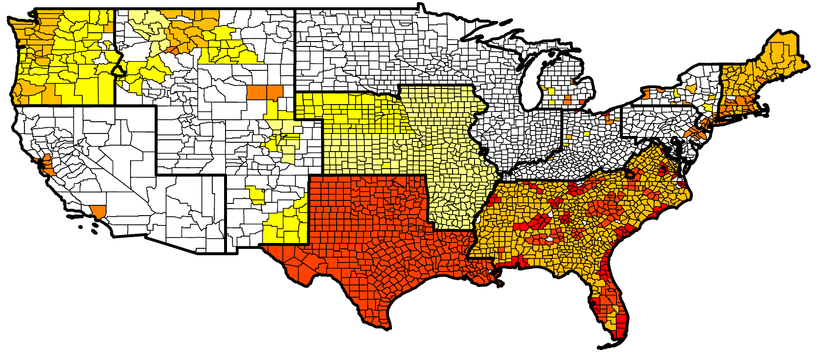
Notes. Darker values represent higher bracket values. Thick black lines mark NWLB regional borders. Counties are unshaded when they were not listed in the brackets or had no stenographers in the 1940 Census. Region I defined brackets at the town level; elsewhere brackets were assigned at the county level.
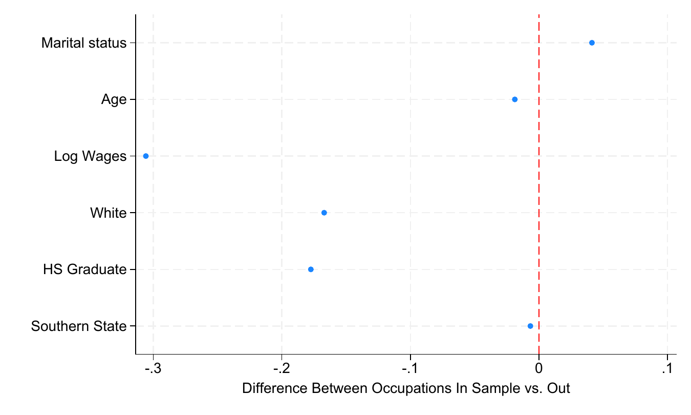
Notes. The sample restrictions follow Goldin and Margo (1992), and counties are restricted to those analyzed in the paper. Differences in means are reported in standard-deviation units. The 95 percent confidence intervals are very small because of the large sample size.
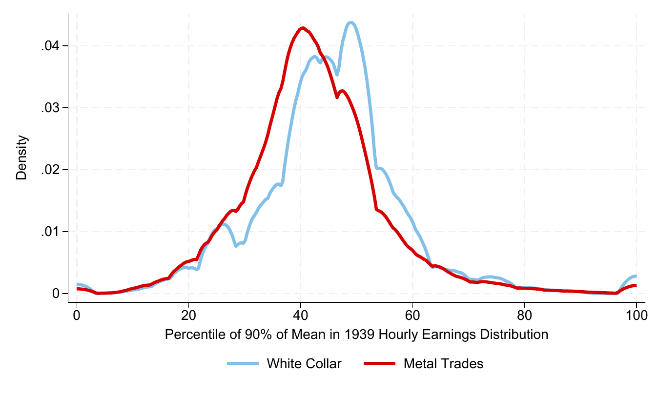
Notes. The figure reports the percentile in the 1939 occupation-by-county hourly-earnings distribution of brackets set to 90 percent of mean earnings. Means are calculated by occupation and NWLB zone. Cells with fewer than three observations are omitted. Hourly earnings use reported labor income and weeks worked, assuming a 40-hour week.
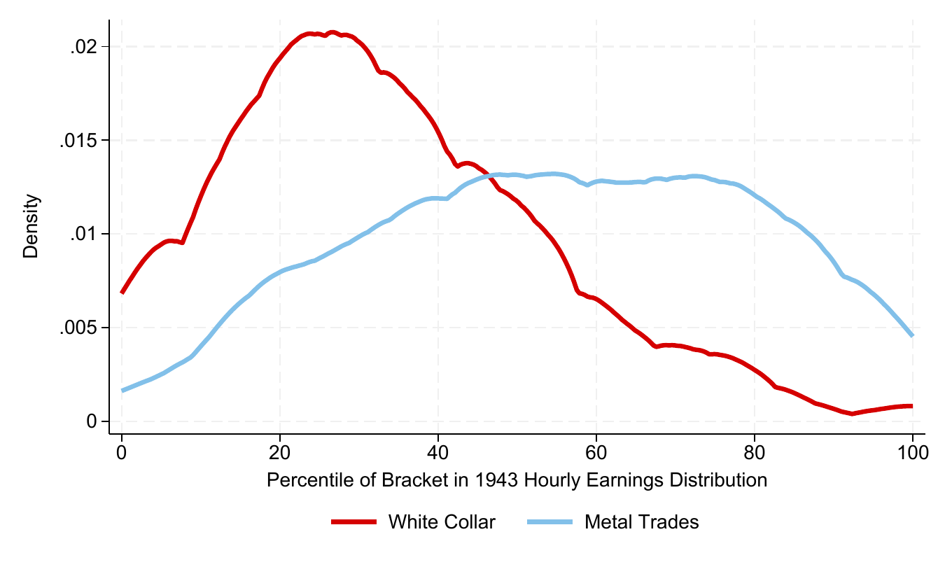
Notes. The figure reports each bracket's percentile in the 1943 hourly-earnings distribution by occupation and county. Cells with fewer than three observations are omitted. The 1943 distribution is imputed from 1939 labor income and weeks worked, assuming a 40-hour week and adjusting for compensation growth from 1940 to 1943.
Linear Term
Quadratic Term
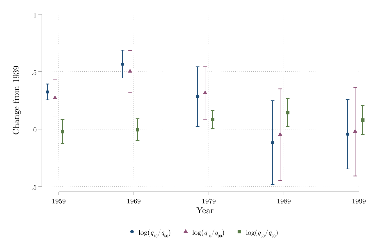
Notes. The unit of observation is an occupation-county. Sample restrictions follow Goldin and Margo (1992). Controls include the 1939 inequality measure and its square, mean labor income, and occupation and county fixed effects. Standard errors are clustered by occupation-county.
Changes in the Log 10–50 Gap
Changes in the Log 50–90 Gap
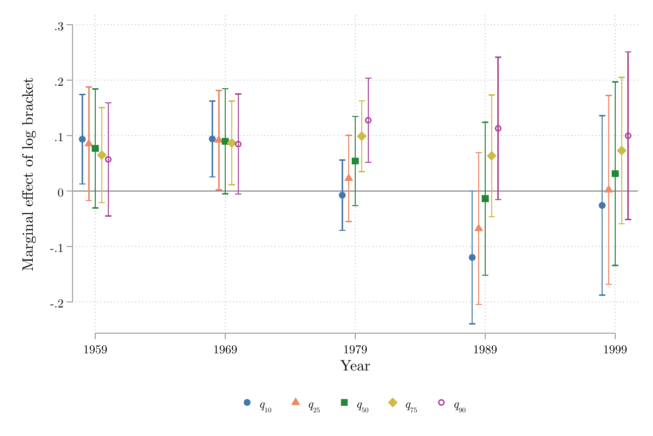
Notes. Marginal effects of an increase in the log bracket are calculated from the estimates in the preceding figure at the 10th, 25th, 50th, 75th, and 90th percentiles of the bracket distribution. Standard errors are calculated as described in the Results section.
Changes in the White–Black Gap
Changes in the High-School Graduate Gap
Notes. The unit of observation is an occupation-county. Sample restrictions follow Goldin and Margo (1992). Controls include the 1939 inequality measure and its square, mean labor income, and occupation and county fixed effects. Marginal effects are calculated at five points in the bracket distribution; standard errors are calculated as described in the Results section.
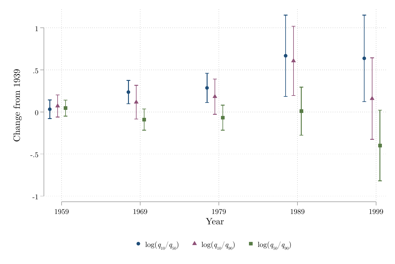
Notes. The unit of observation is an occupation-county. Sample restrictions follow Goldin and Margo (1992). Controls include the 1939 inequality measure and its square, mean labor income, and occupation and county fixed effects. Unionization rates are calculated by state and occupation using Farber et al. (2021) and, where available, the Current Population Survey. Standard errors are clustered by occupation-county.
Evidence
Tables
Table 1Geographic Coverage of the Sample
| Occupation | Counties represented (%) | Individuals represented (%) |
|---|---|---|
| Draftsmen | 2 | 16 |
| Bookkeepers | 58 | 52 |
| Messengers and office boys | 19 | 32 |
| Office machine operators | 13 | 45 |
| Stenographers, typists, and secretaries | 45 | 49 |
| Telephone operators | 24 | 39 |
| Clerical and kindred workers (n.e.c.) | 60 | 47 |
| Carpenters | 29 | 41 |
| Cranemen, derrickmen, and hoistmen | 4 | 22 |
| Electricians | 26 | 40 |
| Machinists | 27 | 49 |
| Millwrights | 14 | 47 |
| Molders, metal | 3 | 25 |
| Painters, construction and maintenance | 4 | 18 |
| Pattern and model makers, except paper | 1 | 13 |
| Tool makers, and die makers and setters | 8 | 58 |
| Furnacemen, smeltermen and pourers | 3 | 16 |
| Heaters, metal | 4 | 19 |
| Oilers and greaser, except auto | 3 | 11 |
| Sawyers | 2 | 7 |
| Truck and tractor drivers | 28 | 37 |
| Welders and flame cutters | 10 | 41 |
| Elevator operators | 3 | 11 |
| Guards, watchmen, and doorkeepers | 28 | 36 |
| Housekeepers and stewards, except private household | 2 | 9 |
| Janitors and sextons | 5 | 24 |
| Practical nurses | 3 | 14 |
| Laborers (n.e.c.) | 29 | 41 |
| Overall | 16 | 31 |
Notes. Sample restrictions follow Goldin and Margo (1992).
Table 2Predicting the Brackets Using the 1943 Hourly-Earnings Distribution
Scroll horizontally to see all specifications.
| Predictor | (1) | (2) | (3) | (4) | (5) | (6) | (7) | (8) |
|---|---|---|---|---|---|---|---|---|
| q₁₀ | 0.226 | -0.021 | -0.017 | -0.006 | ||||
| Standard error | (0.007) | (0.146) | (0.145) | (0.141) | ||||
| q₂₅ | 0.275 | 0.044 | 0.031 | 0.016 | ||||
| Standard error | (0.008) | (0.095) | (0.094) | (0.089) | ||||
| q₅₀ | 0.310 | 0.158 | 0.147 | 0.145 | ||||
| Standard error | (0.007) | (0.095) | (0.095) | (0.093) | ||||
| Mean | 0.321 | 0.139 | 0.132 | 0.121 | ||||
| Standard error | (0.008) | (0.147) | (0.141) | (0.141) | ||||
| Married | 0.090 | 0.101 | ||||||
| Standard error | (0.082) | (0.083) | ||||||
| Age | -0.002 | -0.003 | ||||||
| Standard error | (0.005) | (0.005) | ||||||
| White | 0.282 | 0.281 | ||||||
| Standard error | (0.113) | (0.116) | ||||||
| HS Graduate | -0.086 | -0.060 | ||||||
| Standard error | (0.096) | (0.097) | ||||||
| Combat Supply Contracts | 0.005 | |||||||
| Standard error | (0.002) | |||||||
| Other Supply Contracts | 0.001 | |||||||
| Standard error | (0.001) | |||||||
| Industrial Facilities Spending | -0.001 | |||||||
| Standard error | (0.002) | |||||||
| Military Facilities Spending | 0.003 | |||||||
| Standard error | (0.001) | |||||||
| Unionization Rate | -0.001 | |||||||
| Standard error | (0.002) | |||||||
| Military Inductions | 0.048 | |||||||
| Standard error | (0.019) | |||||||
| Occupation | Yes | No | No | No | No | No | No | No |
| County | Yes | No | No | No | No | No | No | No |
| R² | 0.951 | 0.099 | 0.132 | 0.162 | 0.161 | 0.165 | 0.193 | 0.208 |
| 100 X Ratio of RMSE to Y | 89.000 | |||||||
| Observations | 10625 | 10672 | 10672 | 10672 | 10672 | 10672 | 10672 | 10661 |
Notes. The unit of observation is an occupation-county. Sample restrictions follow Goldin and Margo (1992). The earnings statistics are based on the log 1943 hourly-earnings distribution, imputed from 1939 labor income and weeks worked and adjusted for compensation growth. The five-percent tails are winsorized. Wartime contracts and facilities spending come from ICPSR Study 2896; unionization rates use Farber et al. (2021). Standard errors, shown in parentheses, are clustered by occupation and NWLB zone.
Sources
References
- Acemoglu, Daron, David H. Autor, and David Lyle, “Women, War, and Wages: The Effect of Female Labor Supply on the Wage Structure at Midcentury,” Journal of Political Economy, 2004, 112, 497–551.
- Aizer, Anna, Ryan Boone, Adriana Lleras-Muney, and Jonathan Vogel, “Discrimination and Racial Disparities in Labor Market Outcomes: Evidence from WWII,” 2020. NBER Working Paper 27689.
- Autor, David H., Alan Manning, and Christopher L. Smith, “The Contribution of the Minimum Wage to US Wage Inequality over Three Decades: A Reassessment,” American Economic Journal: Applied Economics, 2016, 8, 58–99.
- ———, Lawrence F. Katz, and Melissa S. Kearney, “Trends in US Wage Inequality: Revising the Revisionists,” Review of Economics and Statistics, 2008, 90, 300–323.
- Bound, John and George Johnson, “Changes in the Structure of Wages in the 1980s: An Evaluation of Alternative Explanations,” American Economic Review, 1992, 82, 371–392.
- Brown, Henry P., The Inequality of Pay, Oxford University Press, 1977.
- Card, David and Alan Krueger, Myth and Measurement, Princeton University Press, 1995.
- ———, Thomas Lemieux, and W. Craig Riddell, “Unions and Wage Inequality,” Journal of Labor Research, 2004, 25, 519–559.
- Collins, William J., “Race, Roosevelt, and Wartime Production: Fair Employment in World War II Labor Markets,” American Economic Review, 2001, 91, 272–286.
- ——— and Gregory T. Niemesh, “Unions and the Great Compression of Wage Inequality in the US at Mid-Century: Evidence from Local Labour Markets,” Economic History Review, 2019, 72, 691–715.
- DiNardo, John, Nicole Fortin, and Thomas Lemieux, “Labor Market Institutions and the Distribution of Wages, 1973–1992: A Semi-Parametric Approach,” Econometrica, 1996, 64, 1001–1044.
- Dube, Arindrajit, The Wage Standard: What's Wrong in the Labor Market and How to Fix It, Penguin, 2026.
- Engbom, Niklas and Christian Moser, “Earnings Inequality and the Minimum Wage: Evidence from Brazil,” American Economic Review, 2022, 112, 3803–3847.
- Etheridge, Bryant, “Contesting the Great Compression: The National Labor Relations Board and Skilled Workers' Struggle to Control Wage Differentials, 1935–1955,” Journal of Policy History, 2020, 32, 183–213.
- Farber, Henry, Daniel Herbst, Ilyana Kuziemko, and Suresh Naidu, “Unions and Inequality Over the Twentieth Century: New Evidence from Survey Data,” Quarterly Journal of Economics, 2021, 136, 1325–1385.
- Ferrara, Andreas, “World War II and Black Economic Progress,” Journal of Labor Economics, 2022, 40, 1053–1091.
- Frydman, Carola and Raven Molloy, “Pay Cuts for the Boss: Executive Compensation in the 1940s,” Journal of Economic History, 2012, 72, 225–251.
- Goldin, Claudia, “The Role of WWII in the Rise of Women's Employment,” American Economic Review, 1991, 81, 741–756.
- ——— and Robert A. Margo, “The Great Compression: The Wage Structure in the United States at Mid-Century,” 1991. NBER Working Paper 3817.
- ——— and ———, “The Great Compression: The Wage Structure in the United States at Mid-Century,” Quarterly Journal of Economics, 1992, 107, 1–34.
- Goldin, Claudia D. and Lawrence F. Katz, The Race Between Education and Technology, Harvard University Press, 2009.
- Hachenburg, Robert, “The National War Labor Board: The Evolution of a National Wage Policy,” University of Pennsylvania Law Review and American Law Register, 1942, 91, 340–357.
- Industrial Union of Marine and Shipbuilding Workers of America, CIO, Research Department, “Rate Determination in the Ship Building and Repair Industry,” December 1951. Manuscript, AFL-CIO Archival Collections, University of Maryland Libraries, College Park, MD.
- Jaworski, Taylor, “You're in the Army Now: The Impact of World War II on Women's Education, Work, and Family,” Journal of Economic History, 2014, 74, 169–195.
- ——— and Gregory T. Niemesh, “Revisiting the Great Compression: Wage Inequality in the United States, 1940–1960,” Historical Methods, 2018, 51, 39–48.
- Juhn, Chinhui, Kevin M. Murphy, and Brooks Pierce, “Wage Inequality and the Rise in Returns to Skill,” Journal of Political Economy, 1993, 101, 410–442.
- Katz, Lawrence F. and Kevin M. Murphy, “Changes in Relative Wages, 1963–87: Supply and Demand Factors,” Quarterly Journal of Economics, 1992, 107, 35–78.
- Keat, Paul G., “Long-Run Changes in Occupational Wage Structure, 1900-1956,” Journal of Political Economy, 1960, 68, 584–600.
- Lee, David S., “Wage Inequality in the United States During the 1980s: Rising Dispersion or Falling Minimum Wage?,” Quarterly Journal of Economics, 1999, 114, 977–1023.
- Levitan, Sar A., “Union Attitudes Toward Job Evaluation and Ingrade Progression,” ILR Review, 1951, 4, 268–274.
- Muntz, Earl E, “The Decline in Wage Differentials Based on Skill in the United States,” International Labor Review, 1955, 71, 575.
- National War Labor Board, “Manual of Going Wage Rates,” Technical Report 1944.
- Officer, Lawrence H. and Samuel H. Williamson, “Annual Wages in the United States, 1774-Present,” 2022.
- Piketty, Thomas and Emanuel Saez, “Income Inequality in the United States, 1913-1998,” Quarterly Journal of Economics, 2003, 118, 1–39.
- Record, Jane Cassels, “The War Labor Board: An Experiment in Wage Stabilization,” American Economic Review, 1944, 34, 98–110.
- ———, “The War Labor Board: An Experiment in Wage Stabilization: Comment: Reply,” American Economic Review, 1944, 34, 575–577.
- Rose, Evan K., “The Rise and Fall of Female Labor Force Participation During World War II in the United States,” Journal of Economic History, 2018, 78, 673–710.
- Rose, Jonathan, “Government Interventions in Times of Economic Crisis.” PhD dissertation, University of California, Berkeley 2009.
- Shatnawi, Dina and Price V. Fishback, “The Impact of World War II on the Demand for Female Workers in Manufacturing,” Journal of Economic History, 2018, 78, 539–574.
- Thurow, Lester, Generating Inequality: Mechanisms of Distribution in the U.S. Economy, Basic Books, 1975.
- United States Department of Labor, The Termination Report of the National War Labor Board, Government Printing Office, 1949.
- Vickers, Chris and Nicolas L. Ziebarth, “Can the Great Compression be Explained by Wartime Wage Controls?,” Explorations in Economic History, 2025, 98.
- Western, Bruce and Jake Rosenfeld, “Unions, Norms, and the Rise in US Wage Inequality,” American Sociological Review, 2011, 76, 513–537.
- Witte, Edwin E., “American Experience with Wage Stabilization,” Wisconsin Law Review, 1952, p. 398.
End matter
Notes
We thank Bob Margo, Ethan Kaplan, Julián Martínez-Iriarte as well as numerous seminar and conference participants for valuable comments. Any views expressed are those of the authors and not those of the U.S. Census Bureau. The Census Bureau’s Disclosure Review Board and Disclosure Avoidance Officers have reviewed this information product for unauthorized disclosure of confidential information and have approved the disclosure avoidance practices applied to this release. This research was performed at a Federal Statistical Research Data Center under FSRDC Project Number 1967 (CBDRB-FY22-P1967-R9320, CBDRB-FY22-P1967-R10073, CBDRB-FY26-P2489-R12947).↩︎
Unfortunately, there are problems with the available 1950 Census microdata in the RDC, which prevents us from using it. The newly released IPUMS full-count version of the 1950 Census has transcription issues with the income variable, which render it useless for our purposes as well.↩︎
Exceptions to this policy were allowed in certain circumstances, but firms were required to formally request approval of such an increase from the Treasury. Frydman and Molloy (2012) report that about 750,000 applications for raise approvals, equivalent to about 30% of covered individuals, were processed between 1942 and 1946.↩︎
Relatedly, Collins and Niemesh (2019) find exposure to unionization mid-century associated with lower inequality even into 2000.↩︎
On unions, see Card et al. (2004), Western and Rosenfeld (2011), and Farber et al. (2021), who all point to the rise and fall in private-sector union membership over the 20th century as a key driver of the swings in inequality.↩︎
On gender, extending the earlier work of Goldin (1991), Acemoglu et al. (2004) use state-level variation in mobilization rates to examine the effect of the war on women’s wages in 1949. Using a similar identification strategy, Jaworski (2014) studies the war’s broader demographic ramifications for women. Shatnawi and Fishback (2018) find a persistent effect on demand for female workers in manufacturing even after the war ends. Consistent with this work, Rose (2018) shows that changes in female employment during the war are driven by demand rather than by the wartime draft reducing the supply of working-age men. On race, Collins (2001) studies the effect of non-discrimination policies in hiring by the federal government. Aizer et al. (2020) examine the effects of military spending contracts while Ferrara (2022) examines variation in the demand for Black labor.↩︎
The discussion in this section borrows from our other work (Vickers and Ziebarth 2025).↩︎
In theory, a “bracket maximum” could be established as well, but this was largely irrelevant as equity adjustments were limited to increasing wages up to the bracket minimum, above which raises were not permitted, and, therefore, “the bracket minimum was of primary significance and in many instances bracket maxima were not established. Bracket maxima were of significance only in ‘rare and unusual’ cases” (United States Department of Labor 1949, 230, volume 1).↩︎
An additional complication was that the bracket minimum, the primary policy instrument, could be expressed either as a single rate or a range, for companies which had variation within an occupation. In this case, “the weighted average rate for an occupation was compared with the single rate” (United States Department of Labor 1949, 236, volume 1). That is, if a plant currently had a range of 60 to 70 cents and the single rate (minimum) bracket was 85 with a range of 80 to 90, the plant could increase its range to 80 to 90. Because the weighted average to be compared to in this case was the single rate, we have used the single rate as our measure of the level of the bracket.↩︎
The NWLB in certain cases also established minimum wages. In Vickers and Ziebarth (2025), we show that the maximum effects of these were much smaller than the maximum effects of the brackets and, for that reason, we ignore the minimum wages in our empirical analysis.↩︎
The closest “precedent” we have for how unlisted industries would have been treated comes from a discussion of “isolated plants” for which there was no explicit bracket coverage either.↩︎
This was a cross-industry occupation, so there was no variation in the bracket by industry.↩︎
The National Archives identifier for these records is 1112364, and the HMS/MLR Entry (i.e., the finding aid record) is PI-78 160.↩︎
We thank Andrew Bossie for alerting us to the existence of this source.↩︎
The top codes for years 1960 through 2000 are respectively $25,000, $50,000, $75,000, $140,000, and $175,000. For 1990, top coded values are reported as the median of incomes for those top-coded within a state. For 2000, the mean income of the state an individual lived in was used as the top code.↩︎
The RDC only has a 1% sample of the 1950 Census long forms as well.↩︎
In the appendix, we document the number of observations dropped by each of these restrictions. We also examine the characteristics of those individuals who earn less than one-half the minimum wage.↩︎
An additional issue in mapping the NWLB records to the Census and the BLS is that even when we can make an exact occupational match between the brackets and these other data sources, in some cases, occupations were further subdivided into, for example, grades (“A”, “B”, and so forth). In these cases, for consistency, we have always selected the “A” grade. Similarly, brackets could be assigned for “senior” and “junior” members of an occupation; we used the senior brackets. We also use the most general occupational category from the brackets available. For example, for clerks (
OCC1950390), we use “general” clerks rather than file or payroll clerks. Finally, we take the “Manufacturing” bracket when there is a division into “departments”.↩︎In some cases, brackets were defined at a sub-county level, which is only an issue in Region I. For these brackets, we aggregate to the county level by weighting town-level brackets by the town population. The Appendix has a detailed analysis on all of the bracket aggregation issues.↩︎
In the appendix, we develop the verbal description here more formally.↩︎
The academic literature on the existence of such spillovers in the case of the minimum wage is mixed. Card and Krueger (1995) as well as Engbom and Moser (2022) provide evidence for such spillovers. On the other side, Autor et al. (2016) argue that these spillovers are simply due to measurement error.↩︎
In the appendix, we show results hold if we use the wage rate instead.↩︎
Rose (2009) includes contemporaneous levels of inequality in his specification, but does not include occupation fixed effects. He argues for including the prior measures of inequality because “the brackets have more opportunity to be low relative to the median if the occupation has a high degree of prior dispersion.”↩︎
Our weighting scheme is slightly different than in Autor et al., who weight by the “sum of individuals’ [in a state] reported weekly hours worked multiplied by CPS sampling weights.” Since we focus on people working at least part-time, the difference between weighting by hours worked versus employment is not a major one.↩︎
In our related paper (Vickers and Ziebarth 2025), we draw on limited contemporaneous wage data and find, in line with the results here, that the brackets were set quite closely to what would have been predicted based on the wage distribution at the time.↩︎
We study this question in more detail in our related paper (Vickers and Ziebarth 2025).↩︎
Hourly earnings were calculated by dividing labor earnings by 40 hours per week times the number of weeks worked.↩︎
Even though \(\log(q_{10}/q_{50})+ \log(q_{50}/q_{90}) = \log(q_{10}/q_{90})\), the effects on the separate components need not add up to the total since we are estimating separate specifications for each.↩︎
The standard error of the marginal effect is equal to the square root of \(SE(\widehat{\beta})^2 + 4 \log \bar{w}^{2} SE(\widehat{\gamma})^2 + 2\textup{cov}(\widehat{\beta},2 \log \bar{w} \widehat{\gamma})\). Because the covariance between \(\widehat{\beta}\) and \(\widehat{\gamma}\) was not disclosed, we use the conservative upper bound by taking the square root of \(SE(\widehat{\beta})^2 + 4 \log \bar{w}^{2} SE(\widehat{\gamma})^2 + 4|\log \bar {w}|SE(\widehat{\beta}) SE(\widehat{\gamma})\).↩︎
A one standard deviation difference is roughly the difference between the median and 90th percentile of the distribution of the brackets.↩︎
Because our sample excludes women, we do not examine effects on the gender earnings gap.↩︎
We do not have any direct evidence on how the brackets were actually enforced by race or other demographic group. Collins (2001) finds that government enforcement of racial nondiscrimination policies during the war were associated with closing racial gaps.↩︎
Even if whites and Blacks worked in completely different occupations, it is still possible for the brackets to reduce the racial gap to the extent that Black occupations had higher levels of inequality before the NWLB. In this case, even if the bracket was set strictly as a function of mean earnings in an occupation, more Blacks would get a raise than whites closing the gap in average earnings between the two groups. Similarly, the effects of the bracket will depend on the skewness of the earnings distribution holding fixed the variance. We explore this mechanism in our companion paper (Vickers and Ziebarth 2025).↩︎
In our related work, we (Vickers and Ziebarth 2025) bound the effects the brackets could have had on within and between inequality in the short-run. We conclude that while the brackets could have reduced within-occupation inequality, their effects on between-occupation (and other dimensions) would have been more limited given how the brackets were set as a function of the preexisting wage distribution.↩︎
Jaworski and Niemesh (2018), in a replication of Goldin and Margo (1992) using enlarged samples, attribute nearly half of the overall change in the 90-10, 90-50, and 50-10 ratios between 1939 and 1949 and 1959 to changes in residual inequality using the Juhn et al. (1993) decomposition. Goldin and Margo (1992), and in the working paper Goldin and Margo (1991), use Bureau of Labor Statistics data to show changes in the wage distribution within occupations before and after the war. For example, the log 50-10 difference fell from 0.230 to 0.190 in iron and steel.↩︎
In the appendix, we show that in the mechanical model, extrapolation based on the marginal effect can be misleading. For example, when the marginal effect on \(\Delta \log q_{10,90}\) is \(0\), suggesting no effects of the bracket due to offsetting effects on \(\Delta \log q_{10,50}\) and \(\Delta \log q_{50,90}\), the level of \(\Delta \log q_{10,90}\) is at its highest possible level for any value of the bracket.↩︎
John T. Dunlop served as the chief of the Research and Statistics Branch of the NWLB and later as Secretary of Labor as well as the Thomas W. Lamont University Professor at Harvard. Building on his experience working for the NWLB, he emphasized throughout his academic career the centrality of internal labor markets in the process of wage determination.↩︎
At least some members of the NWLB also believed that the experience with wage setting during the war would encourage collective bargaining in the future. In the termination report for the NWLB, the statement on Region IV suggested that there was “a more wide-spread appreciation and knowledge of balanced wage structures, job classifications, job descriptions, and of good industrial relations practices, which would be beneficial towards the development of collective bargaining” (National War Labor Board 1944, 663).↩︎
See for example (Dube 2026, Ch. 4) for a discussion of this literature.↩︎
The interaction with white-collar status is imprecisely estimated and not reported here.↩︎
We explain in detail in the appendix how we calculated this measure.↩︎
One puzzling result is the lack of any interaction effect in 1959. One explanation is if the mechanisms of persistence discussed above, such as the war, were sufficient to carry forward the compression of the war into 1959, but afterwards unionization was required for the compression to persist, then the interaction would only become significant in the later period.↩︎
In results we do not report here, we find no relationship between unionization and the brackets and changes either in the white-Black gap or the high school graduate to non-graduate gap.↩︎