Description

Proximity Catch Digraphs

We illustrate PCDs in a two-class setting, extension to multi-class setting can be done in a pair-wise fashion or one-vs-rest fashion for the classes.  For two classes, \(\mathcal X\) and \(\mathcal Y\), of points, let \(\mathcal X\) be the class of interest and \(\mathcal Y\) be the reference class and \(mathcal X_n\) and \(\mathcal Y_m\) be samples of size \(n\) and \(m\) from classes \(\mathcal X\) and \(\mathcal Y\), respectively.

The proximity map \(N(\cdot): \Omega \rightarrow 2^{\Omega}\) associates with each point \(x \in \mathcal{X}\), a proximity region \(N(x) \subset \Omega\). Consider the data-random (or vertex-random) proximity catch digraph (PCD) \(D=(V,A)\) with vertex set \(V=\mathcal{X}\) and arc set \(A\) defined by \((u,v) \in A \iff \{u,v\}\subset \mathcal{X}\) and \(v \in N(u)\). The digraph \(D\) depends on the (joint) distribution of \(\mathcal{X}\), and on the map \(N(\cdot)\). The adjective proximity --- for the digraph \(D\) and for the map \(N(\cdot)\) --- comes from thinking of the region \(N(x)\) as representing those points in \(\Omega\) "close'' to \(x\). The binary relation \(u \sim v\), which is defined as \(v \in N(u)\), is asymmetric, thus the adjacency of \(u\) and \(v\) is represented with directed edges or arcs which yield a digraph instead of a graph. Let the data set \(\mathcal{X}\) be composed of two non-empty sets, \(\mathcal{X}\) and \(\mathcal{Y}\), with sample sizes \(n:=|\mathcal{X}|\) and \(m:=|\mathcal{Y}|\), respectively. We investigate the PCD \(D\), associated with \(\mathcal{X}\) against \(\mathcal{Y}\). Here, we specify \(\mathcal{X}\) as the target class and \(\mathcal{Y}\) as the non-target class. Hence, in the definitions of our PCDs, the only difference is switching the roles of \(\mathcal{X}\) and \(\mathcal{Y}\).

In the PCD approach the points correspond to observations from class \(\mathcal X\) and the sets are defined to be (closed) regions (usually convex regions or simply triangles) based on class \(\mathcal X\) and \(\mathcal Y\) points and the regions increase as the distance of a class \(\mathcal X\) point from class \(\mathcal Y\) points increases.

The Proximity Map Families

We now briefly define three proximity map families.

Let \(\Omega = \mathbb{R}^d\) and let \(\mathcal Y_m=\left \{\mathsf{y}_1,\mathsf{y}_2,\ldots,\mathsf{y}_m \right\}\) be \(m\) points in general position in \(\mathbb{R}^d\) and \(T_i\) be the \(i^{th}\) Delaunay cell for \(i=1,2,\ldots,J_m\), where \(J_m\) is the number of Delaunay cells. Let \(\mathcal X_n\) be a set of iid random variables from distribution \(F\) in \(\mathbb{R}^d\) with support \(\mathcal{S}(F) \subseteq \mathcal{C}_H(\mathcal Y_m)\) where \(\mathcal{C}_H(\mathcal Y_m)\) stands for the convex hull of \(\mathcal Y_m\). In particular, for illustrative purposes, we focus on \(\mathbb{R}^2\) where a Delaunay tessellation is a triangulation, provided that no more than three points in \(\mathcal Y_m\) are cocircular (i.e., lie on the same circle). Furthermore, for simplicity, let \(\mathcal Y_3=\{\mathsf{y}_1,\mathsf{y}_2,\mathsf{y}_3\}\) be three non-collinear points in \(\mathbb{R}^2\) and \(T(\mathcal{Y}_3)=T(\mathsf{y}_1,\mathsf{y}_2,\mathsf{y}_3)\) be the triangle with vertices \(\mathcal Y_3\). Let \(\mathcal X_n\) be a set of iid random variables from \(F\) with support \(\mathcal{S}(F) \subseteq T(\mathcal{Y}_3)\). Let \(\mathcal{U}(T\left(\mathcal Y_3 \right))\) be the uniform distribution on \(T\left(\mathcal Y_3 \right)\). If \(F=\mathcal{U}(T(\mathcal{Y}_3))\), a composition of translation, rotation, reflections, and scaling will take any given triangle \(T(\mathcal{Y}_3)\) to the basic triangle \(T_b=T((0,0),(1,0),(c_1,c_2))\) with \(0 < c_1 \le 1/2\), \(c_2>0\), and \((1-c_1)^2+c_2^2 \le 1\), preserving uniformity. That is, if \(X \sim \mathcal{U}(T(\mathcal{Y}_3))\) is transformed in the same manner to, say \(X'\), then we have \(X' \sim \mathcal{U}(T_b)\). In fact this will hold for data from any distribution \(F\) up to scale.

Spherical Proximity Maps and Associated Proximity Regions

The spherical proximity region of \(x \in T(\mathcal{Y}_3)\) is given by \(N_S(x):=\overline B(x,r(x)) \) where \(\overline B(x,r(x))\) is the closed ball centered at \(x\) with radius \(r(x):=\min_{\mathcal Y \in \mathcal Y}d(x,\mathcal Y)\). Spherical proximity regions give rise to class cover catch digraphs (CCCDs) when open balls are used.

Proportional-Edge Proximity Maps and Associated Proximity Regions

For the expansion parameter \(r \in [1,\infty]\), define \(N_{PE}(x,r)\) to be the proportional-edge proximity map with expansion parameter \(r\) as follows; see also Figure1 below.

Using line segments from the center of mass of \(T(\mathcal{Y}_3)\) to the midpoints of its edges, we partition \(T(\mathcal{Y}_3)\) into "vertex regions" \(R_V(\mathcal Y_1)\), \(R_V(\mathcal Y_2)\), and \(R_V(\mathcal Y_3)\). For \(x \in T(\mathcal{Y}_3) \setminus \mathcal Y_3\), let \(v(x) \in \mathcal Y_3\) be the vertex in whose region \(x\) falls, so \(x \in R_V(v(x))\). If \(x\) falls on the boundary of two vertex regions, we assign \(v(x)\) arbitrarily to one of the adjacent regions.
Let \(e(x)\) be the edge of \(T(\mathcal{Y}_3)\) opposite \(v(x)\). Let \(\ell(x)\) be the line parallel to \(e(x)\) through \(x\). Let \(d(v(x),\ell(x))\) be the Euclidean distance from \(v(x)\) to \(\ell(x)\). For \(r \in [1,\infty)\), let \(\ell_r(x)\) be the line parallel to \(e(x)\) such that \(d(v(x),\ell_r(x)) = rd(v(x),\ell(x))\) and \(d(\ell(x),\ell_r(x)) < d(v(x),\ell_r(x))\). Let \(T_{PE}(x,r)\) be the triangle similar to and with the same orientation as \(T(\mathcal{Y}_3)\) having \(v(x)\) as a vertex and \(\ell_r(x)\) as the opposite edge. Then the proportional-edge proximity region \(N_{PE}(x,r)\) is defined to be \(T_{PE}(x,r) \cap T(\mathcal{Y}_3)\).

Notice that \(r \ge 1\) implies \(x \in N_{PE}(x,r)\). Note also that \(\lim_{r \rightarrow \infty} N_{PE}(x,r) = T(\mathcal{Y}_3)\) for all \(x \in T(\mathcal{Y}_3) \setminus \mathcal Y_3\), so we define \(N_{PE}(x,\infty) = T(\mathcal{Y}_3)\) for all such \(x\). For \(x \in \mathcal Y_3\), we define \(N_{PE}(x,r) = \{x\}\) for all \(r \in [1,\infty]\).  See Ceyhan and Priebe (2005), Ceyhan, Priebe, and Wierman (2006), and Ceyhan (2014) for more detail.

Figure 1. Illustration of the construction of proportional-edge proximity region, \(N_{PE}(x,r=2)\) (shaded region) for an \(x \in R_V(\y_1)\) where \(d_1=d(v(x),\ell(v(x),x))\) and \(d_2=d(v(x),\ell_2(v(x),x))=2\,d(v(x),\ell(v(x),x))\).

Central Similarity Proximity Maps and Associated Proximity Regions

(i) For \(\tau \in (0,1]\), the triangle \(T_{CS}(x,\tau)\) has an edge \(e_\tau(x)\) parallel to \(e(x)\) such that \(d(x,e_\tau(x))=\tau\, d(x,e(x))\) and \(d(e_\tau(x),e(x)) \le d(x,e(x))\) and for \(\tau >1\), \(d(e_\tau(x),e(x)) < d(x,e_\tau(x))\) where \(d(x,e(x))\) is the Euclidean distance from \(x\) to \(e(x)\),

(ii) the triangle \(T_{CS}(x,\tau)\) has the same orientation as and is similar to \(T(\mathcal{Y}_3)\),

(iii) the point \(x\) is at the center of mass of \(T_{CS}(x,\tau)\).

Note that (i) implies the expansion parameter \(\tau\),(ii) implies "similarity", and (iii) implies "central" in the name, (parameterized) central similarity proximity map.
Notice that \(\tau>0\) implies that \(x \in N_{CS}(x,\tau)\) and, by construction, we have \(N_{CS}(x,\tau)\subseteq T(\mathcal{Y}_3)\) for all \(x \in T(\mathcal{Y}_3)\). For \(x \in \partial(T(\mathcal{Y}_3))\) and \(\tau \in (0,\infty]\), we define \(N_{CS}(x,\tau)=\{x\}\). For all \( x\in T(\mathcal{Y}_3)^o\) the edges \(e_\tau(x)\) and \(e(x)\) are coincident iff \(\tau=1\). Note also that \(\lim_{\tau \rightarrow \infty} N_{CS}(x,\tau) = T(\mathcal{Y}_3)\) for all \(x \in (T(\mathcal{Y}_3))^o\),
so we define \(N_{CS}(x,\infty) = T(\mathcal{Y}_3)\) for all such \(x\).

The central similarity proximity maps in Ceyhan and Priebe (2003) and Ceyhan, Priebe, and Marchette (2007) are \(N_{CS}(\cdot,\tau)\) with \(\tau=1\) and \(\tau \in (0,1]\), respectively, and in Ceyhan (2014) with \(\tau>1\).

Figure 2. Illustration of the construction of central similarity proximity region, \(N_{CS}(x,\tau=1/2)\) (shaded region) for an \(x \in R_E(e_3)\) where \(h_2=d(x,e_3^\tau(x))=\frac{1}{2}\,d(x,e(x))\) and \(h_1=d(x,e(x))\).

Delaunay Tessellation

The convex hull of the non-target class \( C_H(\mathcal{Y}) \) can be partitioned into Delaunay cells through the Delaunay tessellation of \( \mathcal{Y} \subset \mathbb{R}^2 \). The Delaunay tessellation becomes a triangulation in \(\mathbb R^2\) which partitions \( C_H(\mathcal{Y}) \) into non intersecting triangles. For the points in the general position, the triangles in the Delaunay triangulation satisfy the property that the circumcircle of a triangle contain no points from \( \mathcal{Y} \) except for the vertices of the triangle. In higher dimensions (i.e., \(d >2)\), Delaunay cells are \(d\)-simplices (for example, a tetrahedron in \(\mathbb{R}^3 \)). Hence, the \( C_H(\mathcal{Y}) \) is the union of a set of disjoint \(d\)-simplices \( \{\mathfrak S_k\}_{k=1}^K \) where \(K\) is the number of \(d\)-simplices, or Delaunay cells. Each \(d\)-simplex has \(d+1\) non-coplanar vertices where none of the remaining points of \( \mathcal{Y}\) are in the interior of the circumsphere of the simplex (except for the vertices of the simplex which are points from \( \mathcal{Y} \)). Hence, simplices of the Delaunay tessellations are more likely to be acute (simplices will not have substantially large inner angles). Note that Delaunay tessellation is the dual of the \emph{Voronoi diagram} of the set \( \mathcal{Y} \). A Voronoi diagram is a partitioning of \( \mathbb{R}^d \) into convex polytopes such that the points inside each polytope is closer to the point associated with the polytope than any other point in \( \mathcal{Y}\). Hence, a polytope \( V(y) \) associated with a point \( y \in \mathcal{Y} \) is defined as \(V(y)=\{v \in \mathbb{R}^d: \lvert v-y \rvert \leq \lvert v-z \rvert \ \text{ for all } z \in \mathcal{Y} \setminus \{y\}\}.\) Here, \(\lvert\cdot\rvert\) stands for the usual Euclidean norm. Observe that the Voronoi diagram is unique for a fixed set of points \( \mathcal{Y}\). A Delaunay graph is constructed by joining the pairs of points in \( \mathcal{Y}\) whose whose boundaries of Voronoi polytopes have nonempty intersections. The edges of the Delaunay graph constitute a partitioning of \( C_H(\mathcal{Y})\) providing the Delaunay tessellation. By the uniqueness of the Voronoi diagram, the Delaunay tessellation is also unique (except for cases where \(d+1\) or more points lying on the same hypersphere). An illustration of the Delaunay tesselation in \( \mathbb{R}^2\) is given in Figure 3 below. More detail on Voronoi diagrams and Delaunay tesellations can be found in Okabe et al. (2000).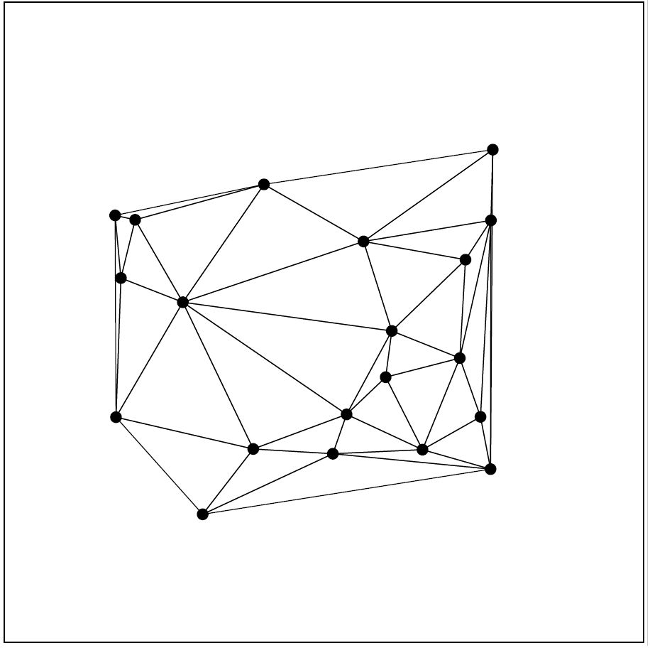

Figure 3. Delaunay triangulation of 20 uniform \(\mathcal Y\) points in the unit square.

Vertex Regions

LLet \( \mathcal{Y}=\{\mathsf{y}_1,\mathsf{y}_2,\mathsf{y}_3\} \subset \mathbb{R}^2 \) be three non-collinear points, and let \( T=T(\mathcal{Y})\) be the triangle formed by these points. Also, let \(e_i\) be the edge of \(T\) opposite to the vertex \(\mathsf{y}_i\) for \(i=1,2,3\). We partition the triangle \(T\) into regions, called vertex regions. These regions are constructed based on a point, preferably a triangle center \(M \in T^o\) where \(T^o\) is the interior of the triangle \(T\). Vertex regions partition \(T\) into disjoint regions (only intersecting on the boundary) such that each vertex region has only one of vertices \( \{\mathsf{y}_1,\mathsf{y}_2,\mathsf{y}_3\}\) on its boundary. In particular, \(M\)-vertex regions are classes of vertex regions, which are constructed by the lines from each vertex \(\mathsf{y}_i\) to \(M\). These lines cross the edge \(e_i\) at point \(M_i\). By connecting \(M\) with each \(M_i\), we attain regions associated with vertices \( \{\mathsf{y}_1,\mathsf{y}_2,\mathsf{y}_3\}\). \(M\)-vertex region of \( \mathsf{y}_i\) is denoted by \(R_M(\mathsf{y}_i)\) for \(i=1,2,3\).  Observe that the interiors of the \(M\)-vertex regions are disjoint. For the sake of simplicity, we will refer \(M\)-vertex regions as vertex regions. An illustration of the \(M\)-vertex regions is given in Figure 4 below.

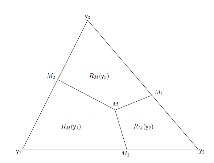
Figure 4. An  illustration of the \(M\)-vertex regions.

Edge Regions

Let \(\mathcal{Y}=\{\mathsf{y}_1,\mathsf{y}_2,\mathsf{y}_3\} \subset \mathbb{R}^2\) be the set of non-collinear points that constitutes some inner triangle \(T=T(\mathcal{Y})\) in \(C_H(\mathcal{Y})\). Let \(e_i\) be the edge opposite to the vertex \(\mathsf{y}_i\) for \(i=1,2,3\). We partition the triangle \(T\) into regions, namely edge regions. These regions are constructed based on a point, preferably a triangle center \(M \in T^o\) where \(T^o\) is the interior of the triangle \(T\). Edge regions are associated with the edges opposite to vertices of \(\mathcal{Y}\). We attain the edge regions by joining each \(\mathsf{y}_i\) with \(M\), also referred to as \(M\)-edge regions. \(M\)-edge region of \(e_i\) is denoted by \(R_M(e_i)\) for \(i=1,2,3\). Observe that the interiors of the \(M\)-edge regions are disjoint. For the sake of simplicity, we will refer \(M\)-edge regions as edge regions. An illustration of the \(M\)-edge regions is given in Figure 5 below.

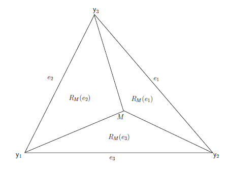
Figure 5. An  illustration of the \(M\)-edge regions.

Minimum Dominating Sets and the Greedy Algorithm

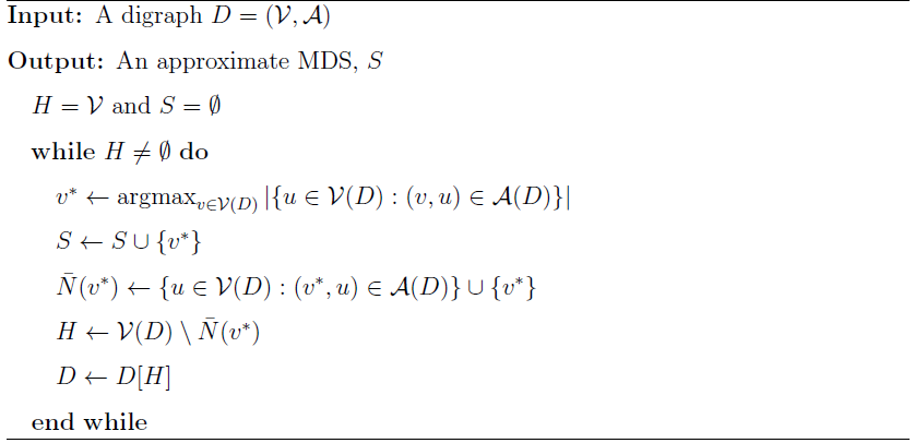
In general, a digraph \(D=(V,A)\) of order \(n=|V|\), a vertex \(v\) dominates itself and all vertices of the form \(\{u:\,(v,u) \in A\}\). A dominating set , \(S_D\), for the digraph \(D\) is a subset of \(V\) such that each vertex \(v \in V\) is dominated by a vertex in \(S_D\). A minimum dominating set (MDS), \(S_{MD}\), is a dominating set of minimum cardinality, and the domination number , \(\gamma(D)\), is defined as \(\gamma(D):=|S_{MD}|\). If an MDS is of size one, we call it a dominating point . Finding an MDS is, in general, an NP-hard optimization problem. However, an approximate MDS can be obtained in \(O(n^2)\) using a well-known greedy algorithm given below. PCDs using \(N(\cdot)=N_S(\cdot,\theta)\) and \(N(\cdot)=N_{CS}(\cdot,\tau)\) are examples of such digraphs. There exists a polynomial time algorithm for finding the MDS (hence for finding the domination number) of PCDs with proximity maps \( N_{PE}(\cdot,r)\), however the existence of polynomial time algorithm for finding the MDS of PCDs with proximity maps \( N_{CS}(\cdot,\tau)\) is still an open problem. \(D[H]\) is the digraph induced by the set of vertices \( H \subseteq V\).

 

References

Ceyhan, E. 2014. “Comparison of Relative Density of Two Random Geometric Digraph Families in Testing Spatial Clustering.” TEST 23(1): 100–134.

Ceyhan, E., and C. E. Priebe. 2003. “Central Similarity Proximity Maps in Delaunay Tessellations.” In Proceedings of the Joint Statistical Meeting, Statistical Computing Section, American Statistical Association.

Ceyhan, E., and C. E. Priebe. 2005. “The Use of Domination Number of a Random Proximity Catch Digraph for Testing Spatial Patterns of Segregation and Association.” Statistics & Probability Letters 73(1): 37–50.

Ceyhan, E., C. E. Priebe, and D. J. Marchette. 2007. “A New Family of Random Graphs for Testing Spatial Segregation.” Canadian Journal of Statistics 35(1): 27–50.

Ceyhan, E., C. E. Priebe, and J. C. Wierman. 2006. “Relative Density of the Random r-Factor Proximity Catch Digraphs for Testing Spatial Patterns of Segregation and Association.” Computational Statistics & Data Analysis 50(8): 1925–64.

Okabe, A., B. Boots, K. Sugihara, and S. N. Chiu. 2000. Spatial Tessellations: Concepts and Applications of Voronoi Diagrams. Wiley, New York.

Maintained by A. Manukyan & E. Ceyhan

Last modified: Oct 16, 2022